There is a famous saying – A topologist is a person who can’t differentiate between a donut and a mug. At the first glance, this might sound very confusing… Donuts and mugs are two very different objects, so how can someone not be able to tell them apart? Well, to realize this joke, we first need to understand homeomorphisms. In this post, we will try to dig deeper into this concept, and then we will talk briefly about surface-to-surface mapping.
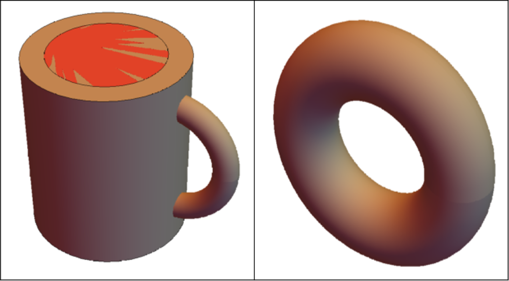
Before diving into the theoretical explanation, let us elucidate the matter with some interesting visualizations. Below is a picture of a basic 3D mug and a donut drawn in Wolfram Mathematica. (Disclaimer: The objects may not look very attractive, but let’s keep it this way for simplification)
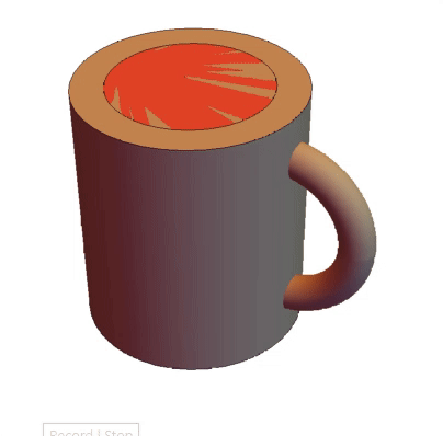
Now, if we look closely, we can change (or deform) the mug into a donut shape. The related code snippet and the deformation are shown below:

We can also go back to our original mug shape from the donut shape. So, we can say that this change is invertible and bijective:

So far, we have seen that we can deform a mug into a donut and vice versa. In other words, we can say there is a map between these two shapes. In mathematical definition, this phenomenon is known as homeomorphism. To be more concise, two shapes are called to be homeomorphic when there is a map between them that is continuous, invertible, and bijective.
Now that we have a basic understanding of homeomorphism, let’s dive deeper into this matter. In the donut and mug example above, we manually designed a deformation function that mapped between these objects. This map will not always work for every other shape we encounter. Moreover, it will be very tedious to manually find every map between all possible pairs of shapes. So, we need to find a generic solution that will work for a larger class of shapes. In geometric terms, this task is commonly referred to as “Surface-to-Surface Mapping”. This task is especially useful for a wide range of geometric applications, such as shape correspondence, texture transfer, layout transfer, and abstract layout embedding.
In the SGP 2021 Graduate School, there was a session titled “Maps Between Surfaces” by M. Campen and P. Schmidt, where the authors described different methods of surface-to-surface mapping in detail. I am deeply intrigued by their talk, and much of the later part of this post has been inspired by their talk.
To understand the concept of surface-to-surface mapping, we need to understand plane-to-plane mapping and surface-to-plane mapping first. In simple terms, plane-to-plane mapping is a homeomorphic map that takes a 2D plane to a different 2D plane. Similarly, surface-to-plane mapping is a homeomorphic map that takes a surface (represented as a triangular mesh) to a 2D plane. But, this might not always be possible for non-disk surfaces. For example, no matter how much we try, a homeomorphic map can’t be found between a 3D sphere and a plane. In such cases, we will use a cut graph to simplify our 3D surface representation.
We are now ready to look at different representation techniques of surface-to-surface mapping:
- Deduction to surface-to-plane mapping (for smooth surface): We can deduce the problem to a simpler surface-to-plane mapping problem. That is, surface A would be mapped to a plane C, and C would be mapped to the other surface, B.
- Vertex to ambient map: In this map, we store the corresponding 3D coordinate of each vertex of surface A.
- Vertex to surface map: Instead of directly storing the 3D coordinate, we store the corresponding triangle ID and relative position on surface B for each vertex of A.
- Vertex to vertex map: For every vertex of surface A, we store a vertex of surface B.
- Functional map: In this setting, we represent the mapping using low-frequency functions (for example, from a Laplacian eigenbasis of the mesh).
However, each of these settings has some disadvantages. The common problem is that all of these maps are only storing information for vertices of A, but not other points on A (such as the points that lie on the edges). Hence, it might be difficult to find the inverse map from surface B to surface A. In other words, these maps are not bijective. For defining perfect homeomorphisms, we can take inspiration from Gauss-Bonnet Theorem. Using this theorem, we can map shapes with 0, 1 and greater than one genus to sphere, plane and hyperbolic plane using Poincare model, Beltrami-Klein model, and hyperboloid model, respectively, so that bijectivity is ensured.
Apart from homeomorphism, a surface-to-surface map must also abide by some other constraints: it has to ensure a low distortion rate, abide by semantic and topological constraints. These constraints can be satisfied by following a two-step approach, consisting of map initialization and map optimization. The authors also described in detail how this approach works. As this is out of the scope of this post, we will not look deeper into those techniques. Interested readers are encouraged to watch their full session here: https://youtu.be/jMWJ79EpyfQ.