Last week I was working on the project “Robust computation of the Hausdorff distance between triangle meshes” under Dr. Leonardo Sacht’s supervision with TA Erik Amezquita and SGI fellows Bryce Van Ross and Deniz Ozbay.
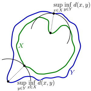
If we have triangle meshes \( A, B \), then \( h(A,B) = \max_{p \in A}d(p,B) \) is called the Hausdorff distance from \( A\) to \( B \), where \(d\) is Euclidean distance. In general case, this function is not symmetric, so the final metric is defined as \(H(a,b) = \max(h(A,B), h(B,A))\).
The Hausdorff distance is very significant in Geometry Processing on the grounds that it may be used for determining the difference between two meshes. The method that we are studying is called the “branch-and-bound” method. The main idea is to calculate the common lower bound for distance from the whole mesh \( A\)to mesh \(B\) and individual upper bounds for distances from every triangle mesh \(T_{A}\) of mesh \( A \) to mesh \(B\). If the upper bounds of some triangles is smaller than the lower bound, then we throw them away and consider the remaining subdivided ones.
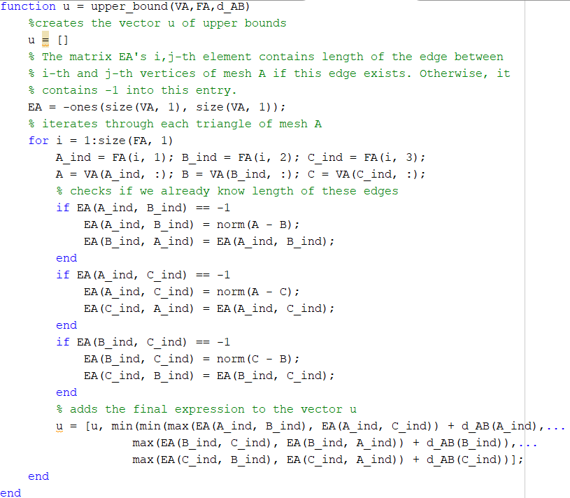
My task was to code the function that returns the upper bounds for distances from every triangle mesh \(T_{A}\) of mesh \( A \) to mesh \(B\). We are going to use the distances between vertices of triangle mesh \(T_{A}\) and triangle inequality to find the upper bound: \[u( T_{A}, B) = \max_{j = 1}^{3}(\max(|v_{j} – v_{j + 1}|, |v_{j} – v_{j + 2}|) + \min_{b \in B}(|v_{j} – b|))\] where \(v_{1}, v_{2}, v_{3}\) are the vertices of triangle mesh \(T_{A}\) .
This is how the implemented algorithm looks like in Matlab:
I really enjoyed working on the project this week with my team, TA and supervisor. I am looking forward to continuing work and improving what we have already done.
For the past two weeks, we have been doing research on how to optimize making 2D cuts onto a surface such that we get an optimal parameterization of the surface onto a disk. This question more generally is asking how we can take a triangulated surface and perform operations on it such that we see a representation of this surface on a disk that we can apply texture mapping or other various changes to.
Firstly let us explain why we want to make these cuts. We make these cuts so that we can use existing methods of disk parameterization from a surface with a boundary onto a disk. We can also think about making a 2D surface from our 3D surface using cuts in a more intuitive way. We can think about it like how a net works, that we know it is true that if we took enough cuts it would be true that we get a locally distortion free 2D representation of the surface; however doing this would both be computationally intensive and not very useful for performing tasks that we want, such as texture mapping, and it does not give an intuitive understanding of what the general surface is or what each section of the 2D map corresponds with each section of the surface. Thus the question becomes how do we take a minimal amount of cuts such that we have a 2D parameterization of the surface that minimizes distortion such that we can still use it for various texture mapping applications.
Disk Parameterization:
First we worked on mapping 3D meshes with existing boundaries to a disk. We implemented existing methods of disk conformal parameterization using three different weight functions. We start by mapping the mesh boundary to the circle, preserving the distance between chord edges. Placing the interior points is then a matter of solving a system of linear equations. In our first weighting method, each edge is weighted the same so in the resulting disk, interior points are the centroid of their neighbors. This gives one linear equation for each interior point, and since the boundary points are fixed, we can solve for the exact locations of each point on the disk.
Weighing each edge uniformly results in unnecessary distortion. Our second and third methods use the angles in the faces sharing the edge to add weights to the equations in the first method. The second method uses harmonic weights, with formula \(w_{i,j}=\frac{1}{2}\left( cot(i,j) + cot(i,j)\right)\) where \(\alpha_{i,j}\) and \(\beta_{i,j}\) are the angles opposite the edge connecting the \(i\) and \(j^{th}\) vertices. These weights reduce distortion, but obtuse angles can result in negative weights, so the resulting map is not guaranteed to be bijective. The third method, mean value weights, resolves this by instead using \(w_{i,j}=\frac{tan(\frac{\gamma_{i,j}}{2}) + tan(\frac{\delta_{i,j}}{2})}{2|| v_i – v_j ||}\) where \(\gamma_{i,j}\) and \(\delta_{i,j}\) are the angles adjacent to the edge connecting the \(i\) and \(j^{th}\) vertices. In our future disk parameterizations, we use these last two methods.
Methods 1, 2, and 3 from left to right
Virtual Boundary:
A downside to disk parametrization is that because the boundary has a fixed mapping to the circle, the resulting parameterization has a lot of distortion near the perimeter. There are a variety of free-boundary parameterization methods, but we focused on the virtual boundary method. By adding one or more layers of faces to the existing boundary, we create a new, virtual boundary that is mapped to the circle while the real boundary is allowed a less constrained shape. We can then ignore the added faces and use the resulting parameterization. The more layers in the virtual boundary, the more “free” the resulting boundary. For example, the mountain range mesh below has a boundary that is more rectangular in shape than circular. As we add more layers to the virtual boundary parameterization, we can see the outline become more square as well.
1 Layer
5 Layers
10 Layers
However, it is not always necessary to add multiple layers, but instead simply increase the size of the virtual boundary, this is due to how the virtual boundary is created following the method used in “Parametrization of Triangular Meshes with Virtual Boundaries” by Yunjin Lee, Hyoung Seok Kim, and Seungyong Lee. We create the virtual boundary by listing the vertices in the existing boundary as \(v_1,v_2,\dots,v_n\) and label the vertices in the virtual boundary \(v’_1,v’_2,\dots,v’_{2n}\) where \(v_i\) corresponds to \(v’_{2i}\), we then make sure the distance between \(v_i , v_{i+1} \) proportional to the distance between \(v_{2i} , v_{2i+2}\) and assigning \(v_{2i+1}\) to the midpoint between the two, to do this we simply say that \(v_{2i}=av_i\). Thus we can increase the size of the virtual boundary simply by increasing the a value, this allows a quicker method of getting a virtual boundary that gives the same results as running multiple layers of virtual boundaries.
a = 1.05
a = 1.5
Many meshes that we want to parameterize in 2D do not have boundaries. In order to do this, we make a cut along existing edges in the mesh to create our own boundary. A cut can be visualized as exactly how it sounds—taking a pair of scissors and slicing through the mesh. It is created from a path of edges by duplicating the non-endpoint vertices in the path, and connecting them to create a loop of boundary edges. This connected loop will naturally form by reassigning the faces on one side of the path to contain the new vertices rather than the old duplicated vertices.
The trouble comes with determining which side of the cut each face is on. We created our own cutting algorithm, and solved this problem by using the orientation of the faces with edges on the path. Given a directed path, the faces with edges on one side of the path will be oriented in the direction of the path, while the faces on the other side will be oriented in the opposite direction. Thus we can easily separate the faces sharing edges along the cut. A more difficult task is separating the faces that only share one vertex with the cut path. To solve this quickly, we store the directions of edges coming from each point on the path that are confirmed to be on one side of the path. We then can determine which side of the path a face is based on how close its edges’ direction is to these edges. There are conceivable shares which will cause this to fail, but in practice this can quickly implement the vast majority of cuts.
We also tried a different algorithm to determine which side of the cut each face is on, making use of geometric properties of the surface, in specific the normal of the surface. We compared the normal of the face to the normal of the edge on the cut. We took the plane defined by the normal on the cut, and compared if the normal of the face projected onto the plane was on the left or right of the plane, when considering the y-axis of the plane to be the edge. This result showed initial success, and continuous to work along small cuts, or cuts along areas of low curvature, however when dealing with areas of large curvature the cut has a large issue, that is when the surface has high curvature it is possible for the edge to be behind the surface with respect to where the edge is, which gives the normal on the other side than we desire, and thus gives it to be on the right when it is on the left, and other such issues, for this reason we have discarded this approach, however we are open to the possibility that using some operation on the normals it might be possible to use this approach.
Euclidean Max Cut:
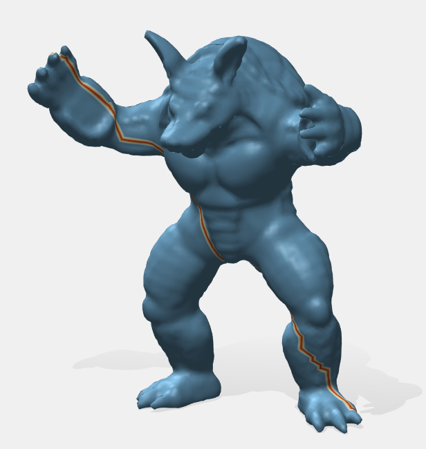
Now let us discuss our main method of how to choose a cut to make, we considered existing methods, namely the method of using a minimal spanning tree as used by Alla Sheffer in “Spanning Tree Seams for Reducing Parametrization Distortion of Triangulated Surfaces,” seemed to have the opposite desire than we want, that is, to minimize the size of the cut. It is clear simply from the boundaries we were provided as well as intuition that the larger the cut the smaller the distortion would be, as if we had a large enough cut there would be no distortion, however we also know that artifacts exist along the cuts, thus we created a new method. This method was a way of maximizing the distance of the cut while minimizing the artifacts. This was maximizing the Euclidean distance between the end points of the path of the cut while making the cut that takes the minimum geodesic distance.
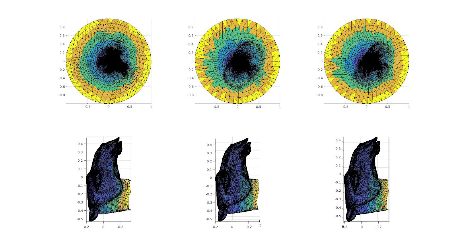
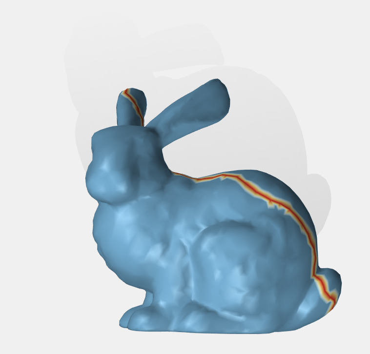
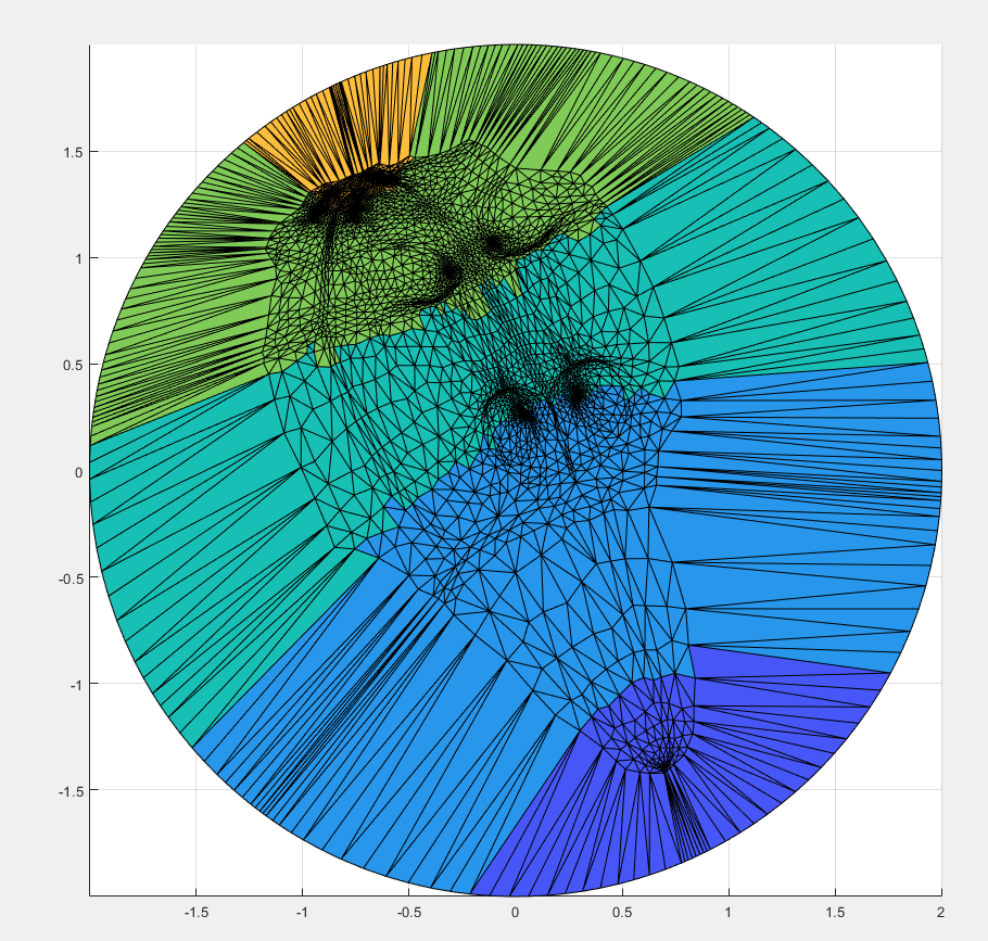
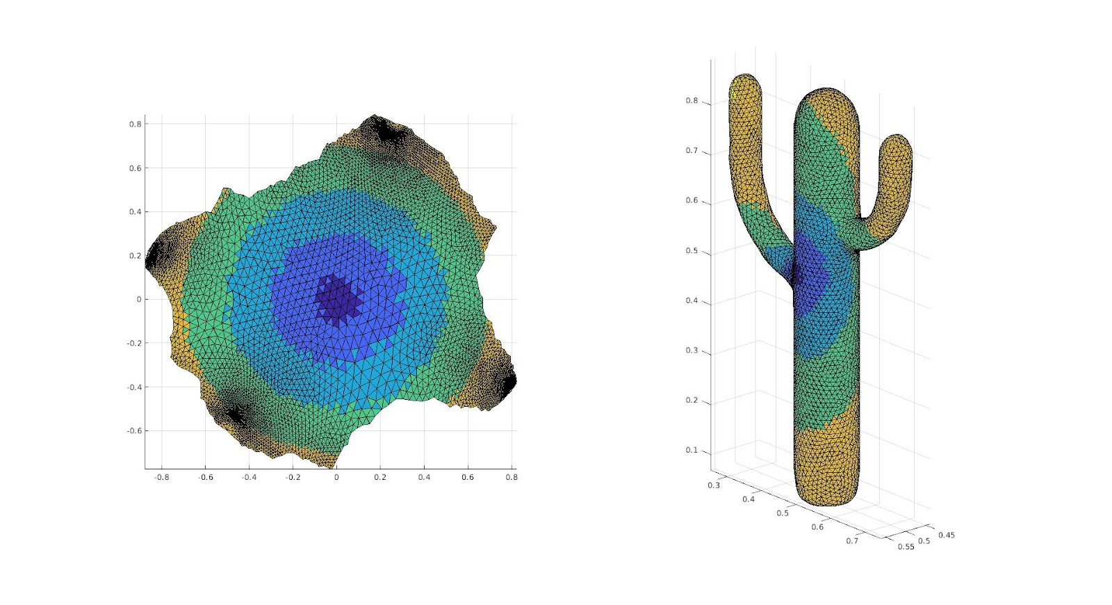
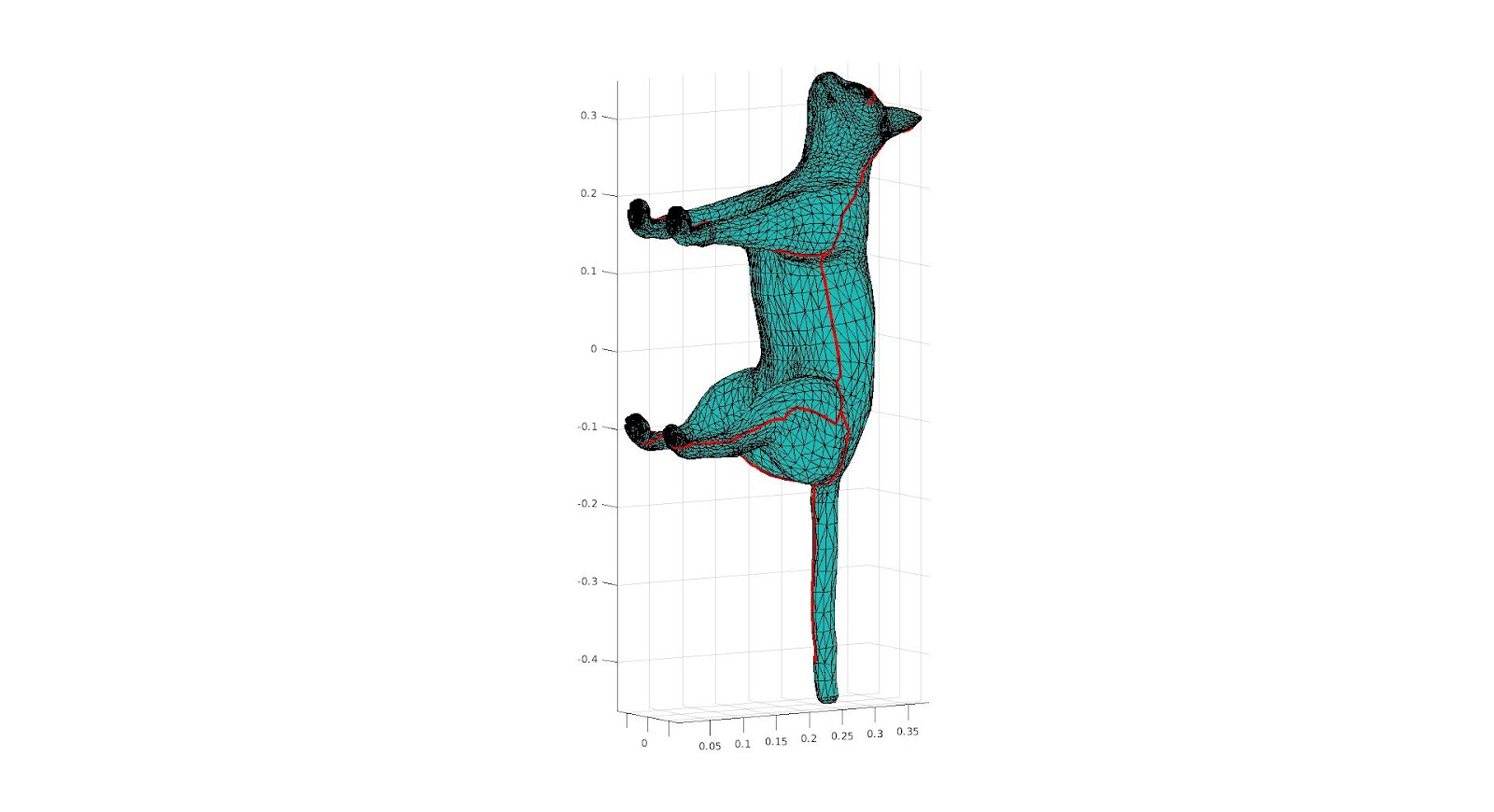
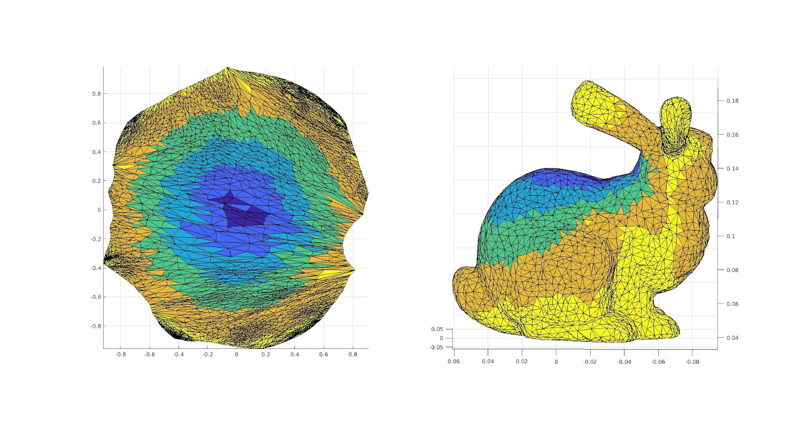
The surface, and the cut we are making upon it.
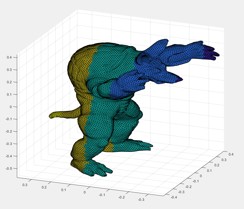
A color function we add to the surface in order to see where different areas are mapped onto a 2D Parameterization.
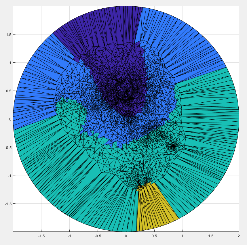
The 2D Parameterization with Virtual Boundary.
The surface, and the cut we are making upon it.
A color function we add to the surface in order to see where different areas are mapped onto a 2D Parameterization.
The 2D Parameterization with Virtual Boundary.
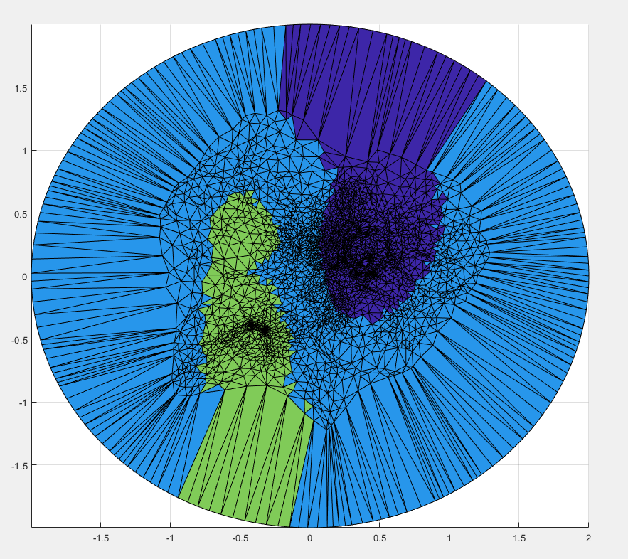
The surface, and the cut we are making upon it.
A color function we add to the surface in order to see where different areas are mapped onto a 2D Parameterization.
The 2D Parameterization with Virtual Boundary.
The surface, and the cut we are making upon it.
A color function we add to the surface in order to see where different areas are mapped onto a 2D Parameterization.
The 2D Parameterization with Virtual Boundary.
As we can see however this creates unintuitive cuts, and cuts that do not have our desired purpose, for this we considered a new method of cuts.
Medial Mesh Max Cut:
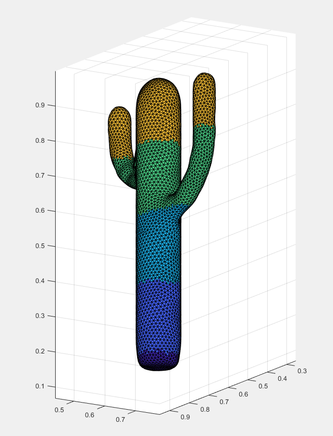
To deal with this issue, we implemented a new method using the medial mesh, that is we consider a simplified mesh of the object making use of the midpoints of the faces within the interior of the surface. We did not do implementation of finding this medial mesh ourselves, rather using the code created in “Q-MAT: Computing Medial Axis Transform by Quadratic Error Minimization” by Pan Li, Bin Wang, Feng Sun, Xiaohu Guo, Caiming Zhang and Wenping Wang. We then after obtaining the Medial Mesh, create the minimal spheres on each vertex, that is the smallest sphere with the center at a vertex in the medial mesh, such that it intersects with a vertex on the surface. We then created a graph with vertices representing the spheres, and creating an edge if the spheres overlap, we then calculated the maximum path existing on the graph, with the edge lengths equal to the distance between the center of the spheres. We then identified the vertices on the surface such that they were the closest to the points on each sphere such that the Euclidean distance between the two end point spheres is maximized, we use these as the two points to create a cut on and we create a cut with the minimum geodesic distance between the two points. This was hopefully to avoid areas of high curvature, and thus create a better cut still of a reasonably large size.
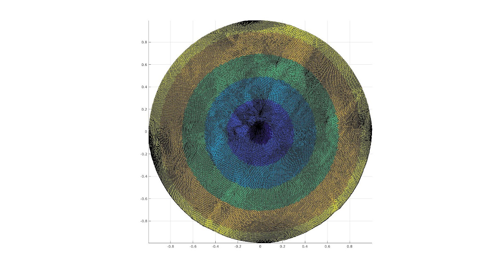
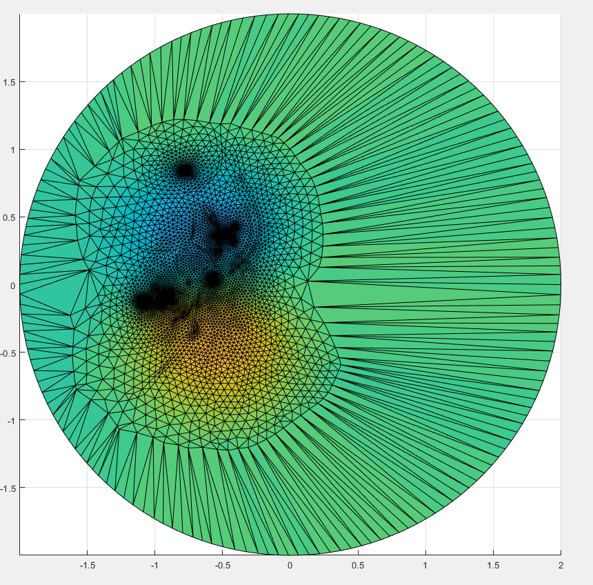
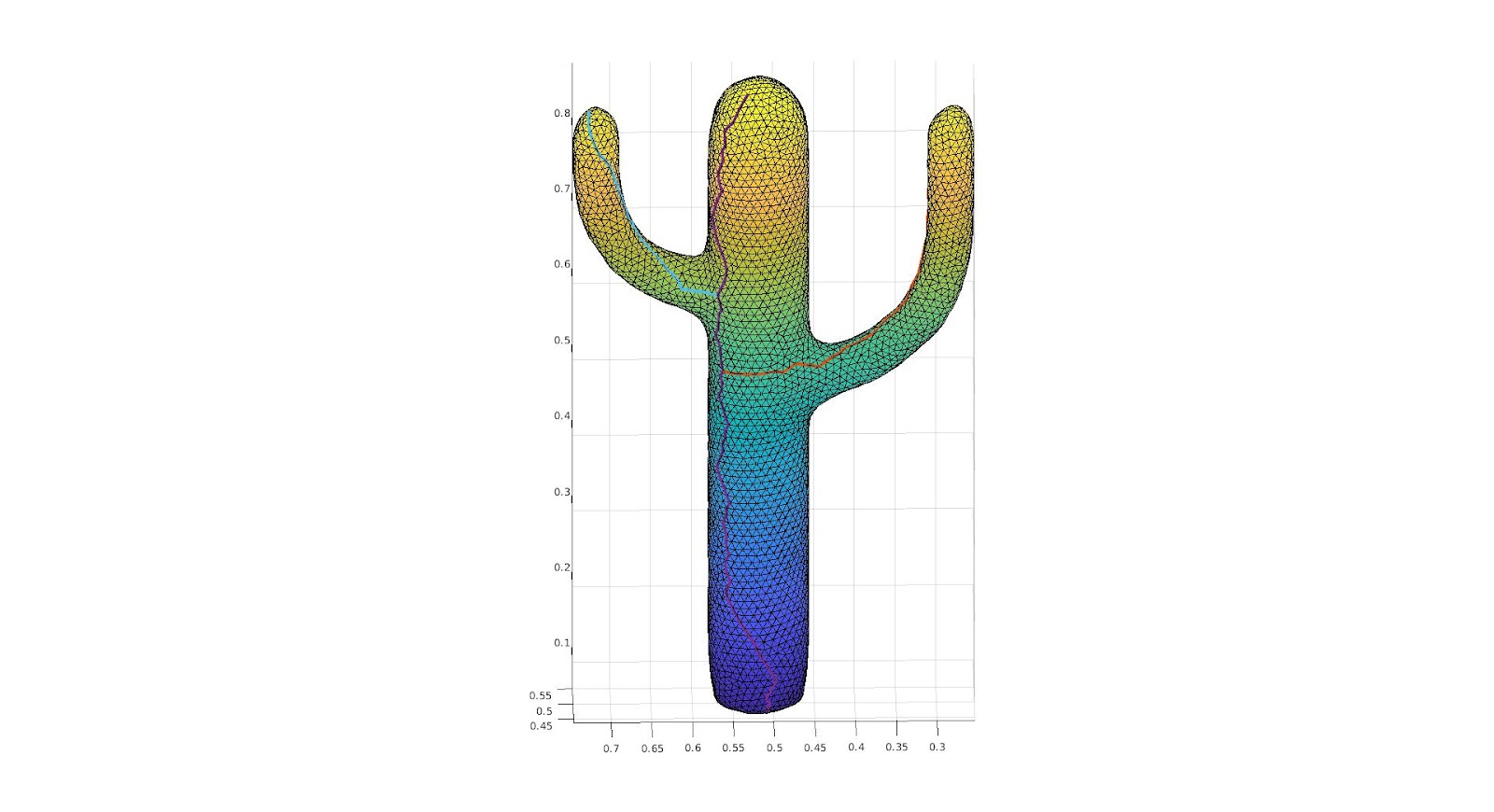
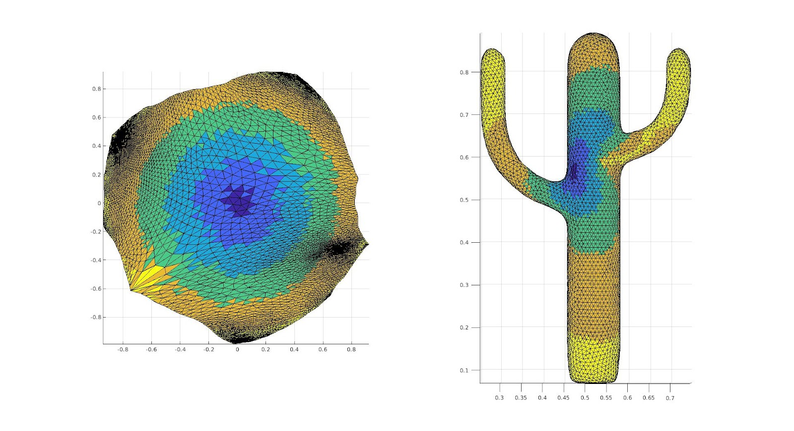
The surface, and the cut we are making upon it.
A color function we add to the surface in order to see where different areas are mapped onto a 2D Parameterization.
The 2D Parameterization with Virtual Boundary.
The surface, and the cut we are making upon it.
A color function we add to the surface in order to see where different areas are mapped onto a 2D Parameterization.
The 2D Parameterization with Virtual Boundary.
The surface, and the cut we are making upon it.
A color function we add to the surface in order to see where different areas are mapped onto a 2D Parameterization.
The 2D Parameterization with Virtual Boundary.
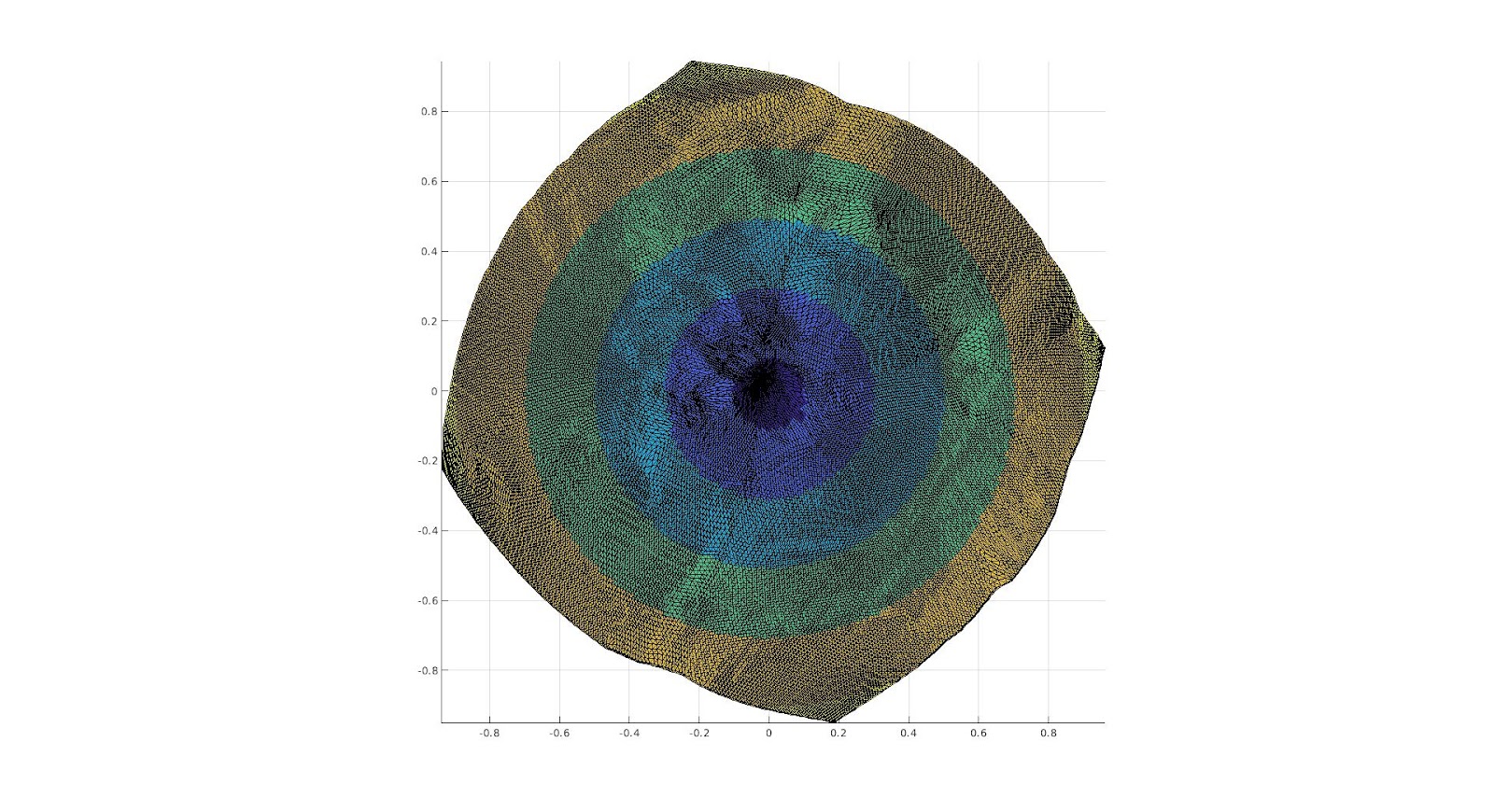
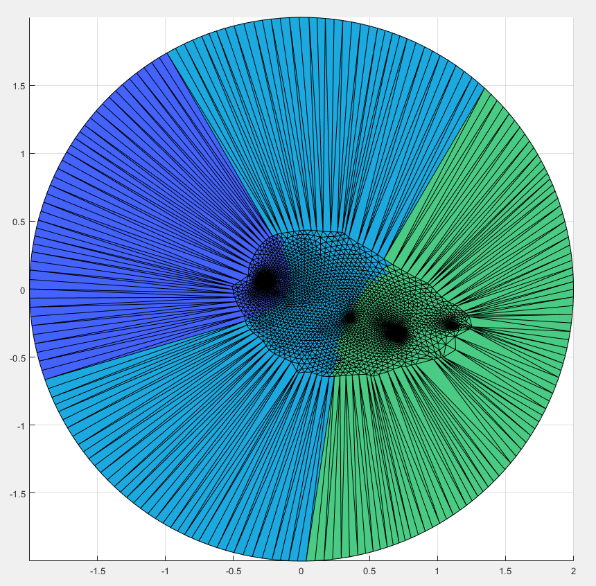
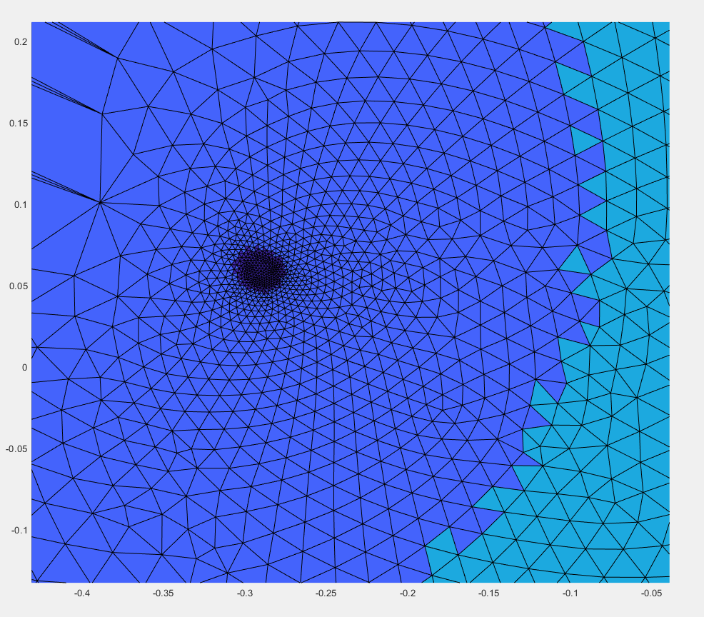
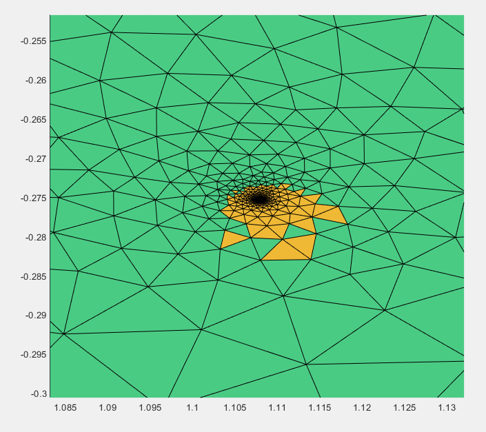
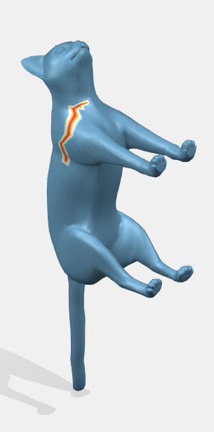
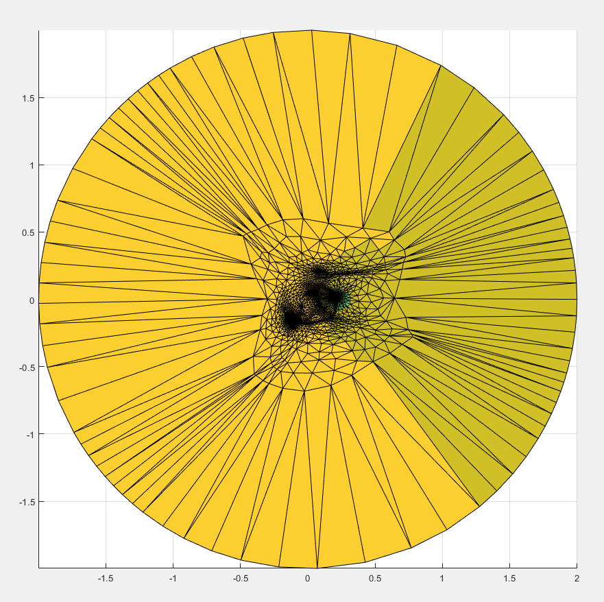
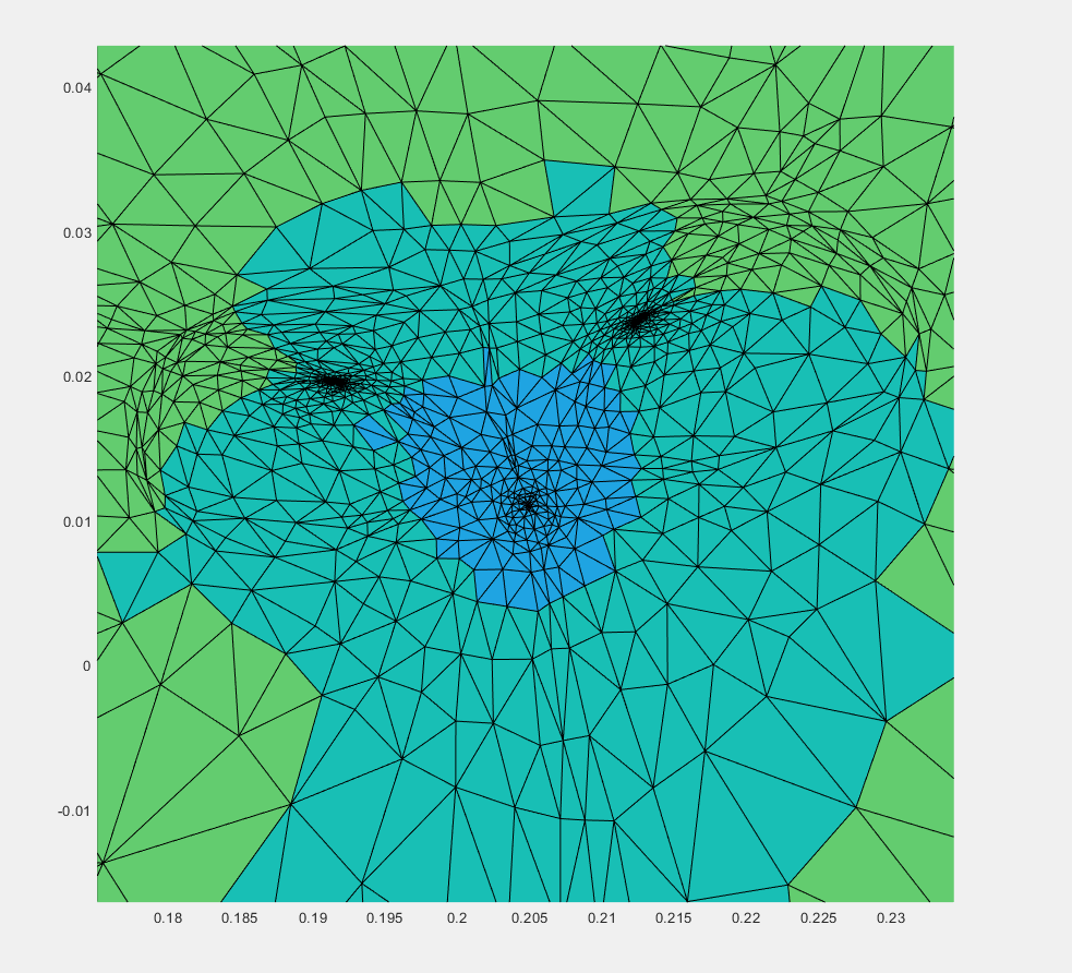
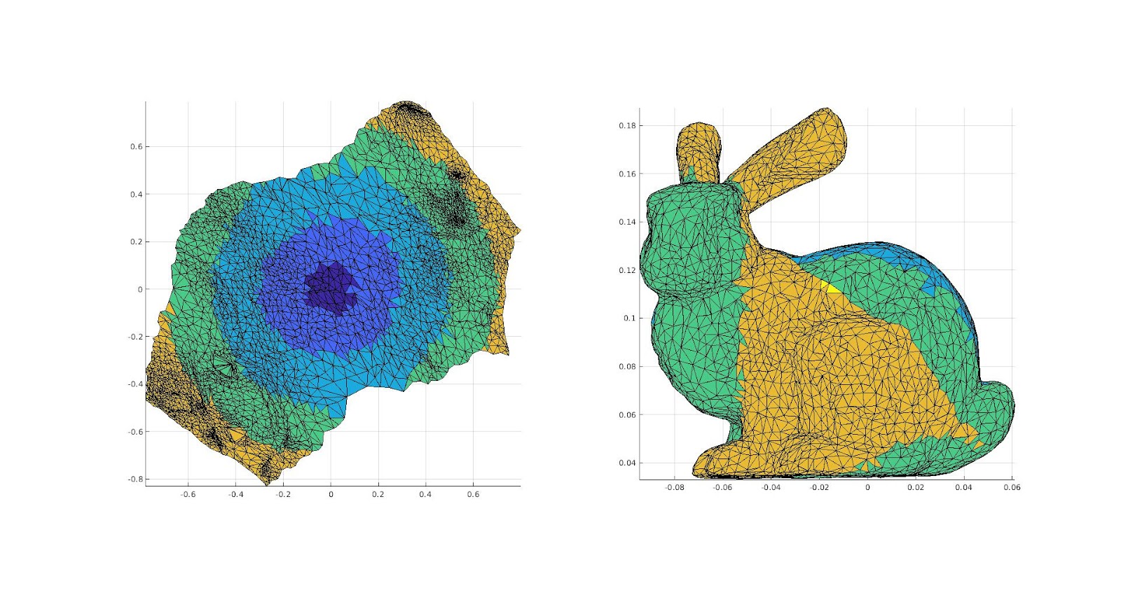
Of note is that areas that are not on the cut area directly are “tucked in” so to into the areas that we can barely see. The one below is in the left area with a high density of vertices. The rest follow from left to right the areas of high vertices.
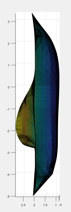
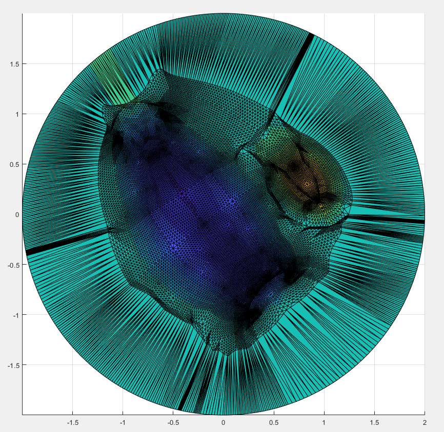
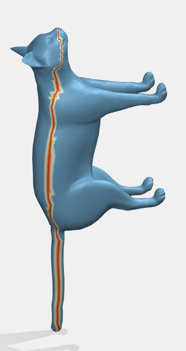
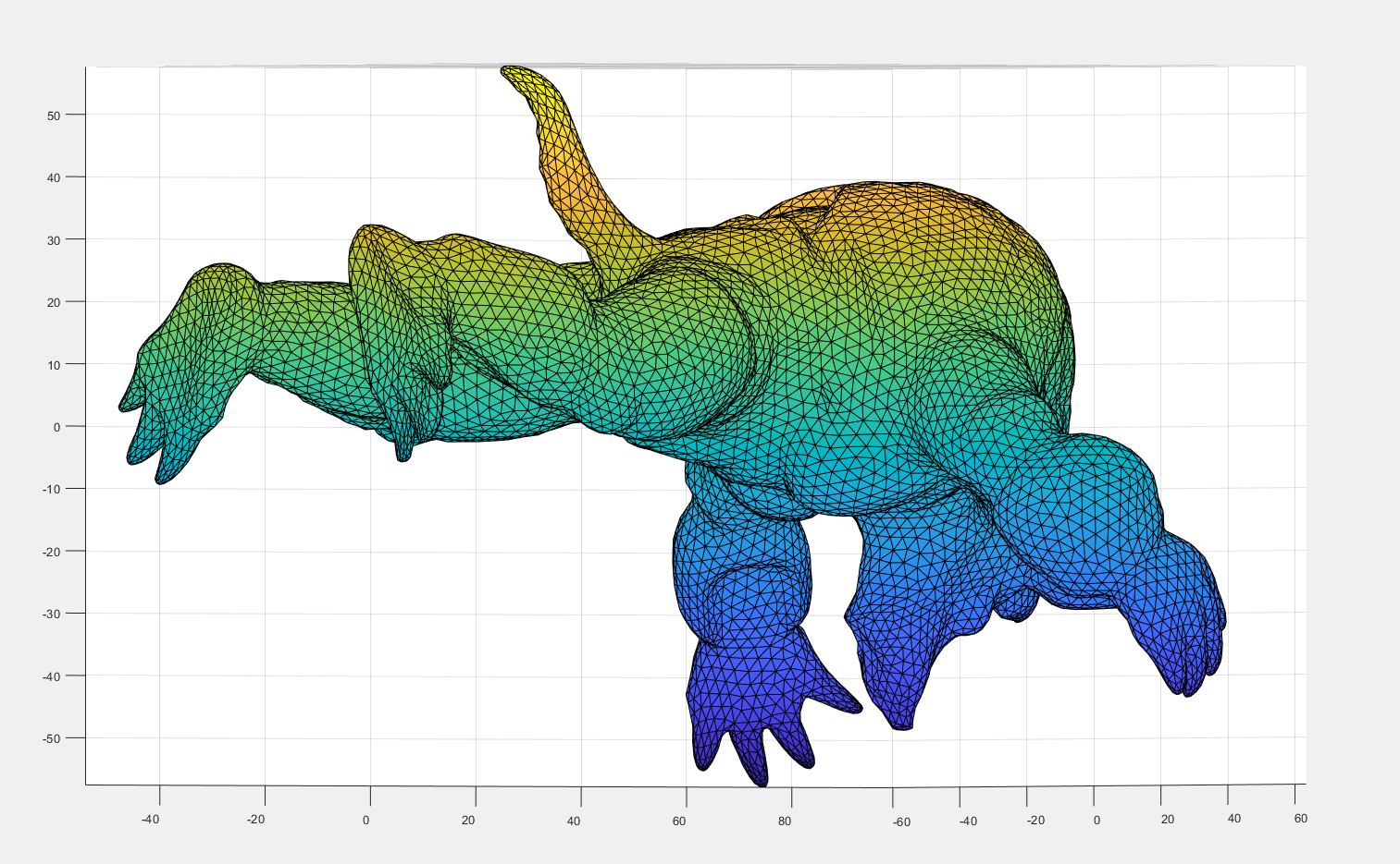
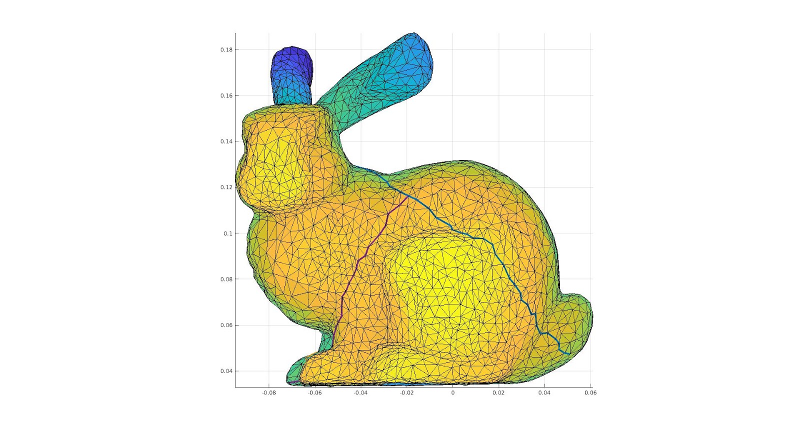
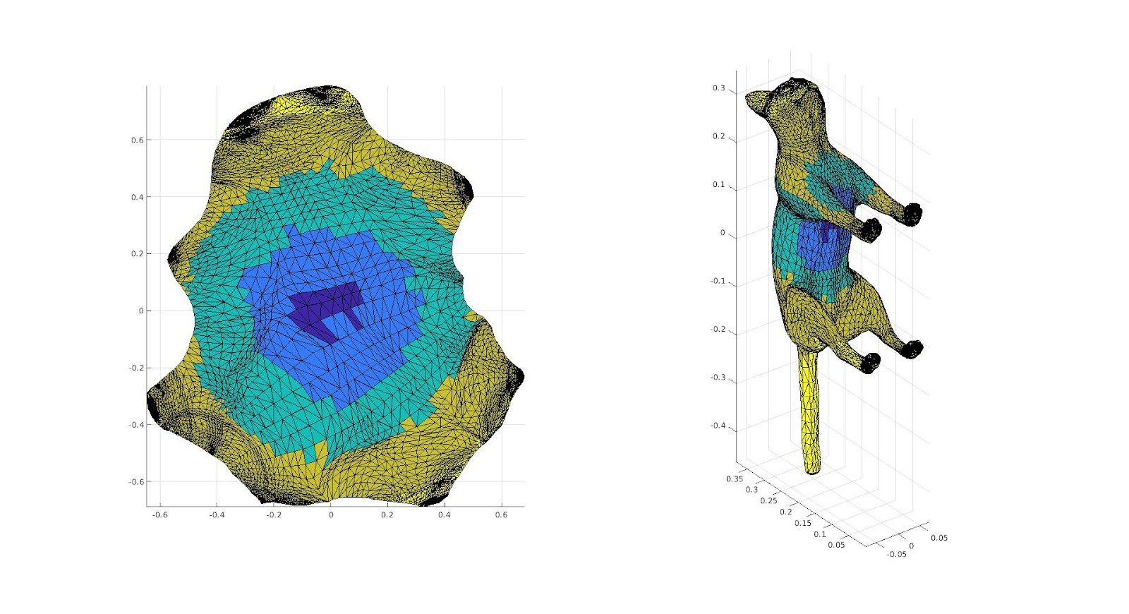
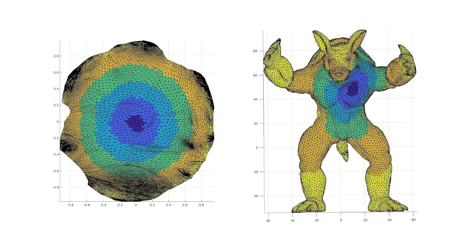
The surface, and the cut we are making upon it.
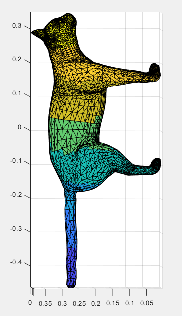
A color function we add to the surface in order to see where different areas are mapped onto a 2D Parameterization.
The 2D Parameterization with Virtual Boundary.
We again get areas of high curvature being sort of tucked into the surface.
The bottom left area that shows the face.
The right middle area showing the back legs and tail.
How Multiple Cuts work:
Thus far we have only discussed and shown single cuts along simple paths. It is also possible, and often preferred, to make multiple cuts on intersecting paths. Making these cuts sequentially, each new cut is equivalent to making a cut on a shape that already has a boundary. If the cut path has one endpoint on the boundary and the rest of the points on the interior, then the resulting boundary is still a simple closed path, as is necessary for our 2D parameterization. The method is the same as before, except the endpoint on the existing boundary is duplicated in addition to the other points. Using multiple cuts increases the freedom of our cut paths and allows us to cut along branching pieces of a mesh.
We can extend our previous Euclidean maximum cut method to multiple cuts in an iterative process. After making our first cut as usual, we repeat the same method but restricting one of the endpoints to be on the previous cuts. Our second cut selects the point that is farthest from our new boundary and chooses the shortest path between them. This is repeated until there are the desired number of cuts. Below are some examples of multiple cuts using this method. One possible automated method of stopping would be to calculate the standard deviation of the distance from the boundary and continue to create cuts until it is below some threshold.
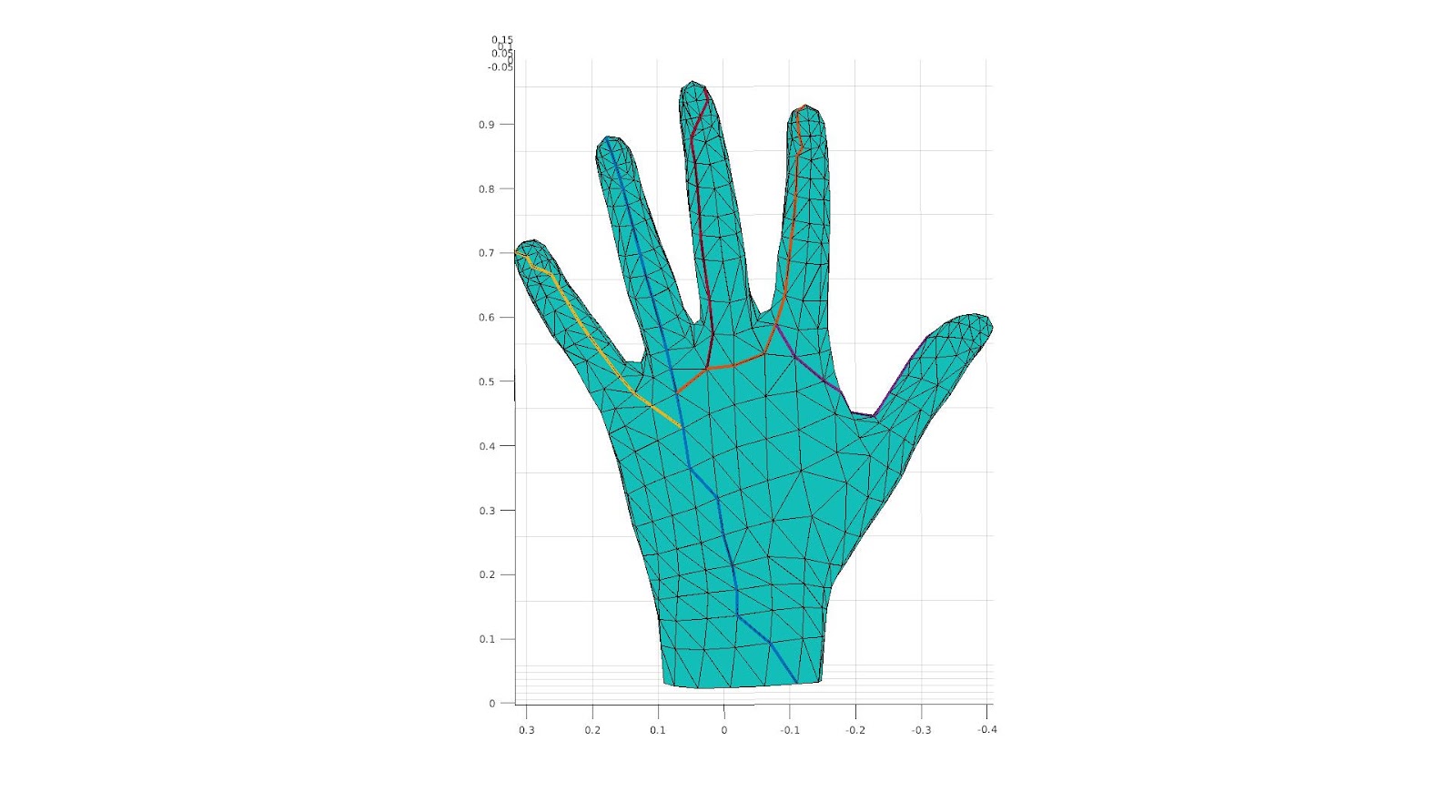
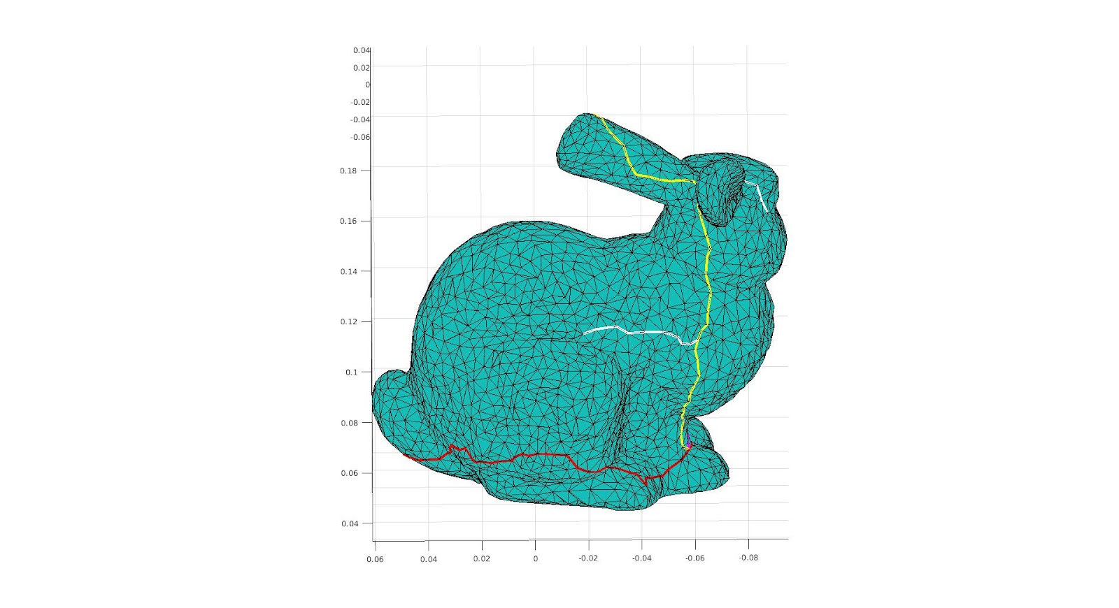
The surface, and the cuts we are making upon it.
The 2D Parameterization and a color function that we take from 2D parameterization to the surface.
The surface, and the cuts we are making upon it.
The 2D Parameterization a color function that we take from 2D parameterization to the surface.
The surface, and the cuts we are making upon it.
The 2D Parameterization a color function that we take from 2D parameterization to the surface.
[example of cutting through diagonals and where we don’t want, downside of this method]
We can also use the sphere approximation to make multiple cuts. The spheres’ centers indicate important spots in the mesh, like joints and protrusions. We decided to use a minimum spanning tree to determine a sequence of cuts that connects each of these areas. First we project each sphere center to a vertex on the mesh. Then we make a weighted graph out of these points where an edge between two points is weighted as their geodesic distance. This graph gives a minimum spanning tree that can be broken into a sequence of cut paths that connects each point from our sphere approximation. The paths sometimes require simple adjustments to remove overlap, and then they are ready for our cutting algorithm.
The surface, and the cuts we are making upon it.
The 2D Parameterization a color function that we take from 2D parameterization to the surface.
The surface, and the cuts we are making upon it.
The 2D Parameterization a color function that we take from 2D parameterization to the surface.
The surface, and the cuts we are making upon it.
The 2D Parameterization a color function that we take from 2D parameterization to the surface.
The surface from the front, and the cut we are making upon it.
The surface from the back, and the cuts we are making upon it.
The 2D Parameterization a color function that we take from 2D parameterization to the surface.
Conclusion:
This research was very interesting, but we did not get the sort of success that we would like: While we did get surfaces with minimal distortion, specifically those with multiple cuts, we did not get the desired usage that we would like. Thus it is necessary to state what future direction should be taken if this research would be continued. There are three main areas for future work.
The first is making cuts along lines that preserve symmetry, that is if the surface has symmetry along some axis, or some feature, the 2D parameterization also has these symmetries. This would be useful both for minimizing the distortion and would provide intuitive results for texture mapping. These lines of symmetry, however, would be incredibly difficult to calculate, so we would like for them to be usually user specified, which brings us to the second area: how the inclusion of landmark areas would be useful, that is specifying areas where the cut cannot travel through. This allows us to intuitively avoid areas of high curvature that are important to the surface and how it could be applied to different surfaces as useful for an artistic application.
We could also try to do this in an automated way by using a skeletal approximation of the surface, using either a simplified medial mesh or a method presented in the SGP 2021 Graduate School Course Shape Approximations & Applications: using the sphere mesh proxy simplification of a surface. This method considers the edges between the spheres as the “bones” and makes a cut on each bone section such that it goes over the entirety of the bone, but avoids areas of high curvature by making minimal geodesic cuts along each bone; the method connects the bones by paths the minimize the total geodesic distance. A secondary way to use this is to make cuts along the “bones” but additionally taking a cut perpendicular to the bone at each point where the sphere begins. To think of this on a 3D model of a cat, for example, we would take a cut along the spine, and then take a perpendicular cut along the cat. To see if either of these methods work and if so which is better, further research would be needed.
AKA: Takeaways from Weeks 1-2 of High-order Directional Field Design Research
Author: Bryce Van Ross
It’s incredible how much one can learn in a month, and I’m looking forward to learning more (especially theoretically). In that same spirit, I highlight some takeaways from research made in my first SGI project. This project was guided by research mentor Dr. Amir Vaxman and TA Klara Mundilova, where I worked with fellow SGI student Jonathan Mousley.
Question(s): Usually we think of vectors and computations like divergence and curl as interrelated, and they are. But can we determine something more nuanced about these properties with respect to some vector field if we encounter a complex (i.e. having multiple vertices/edges) triangular mesh? Yes, we can. But it depends on your choice of approach of partitioning your mesh. For the sake of my research, we focus on the face-based representation.
Face-based representations of vector fields can then be broken down into vertex-based and edge-based approaches, per face per triangle. This means we are working with vector fields on faces that are gradients of (piecewise linear) functions that are either defined on the vertices or on the midpoints of edges. Depending on the choice of approach, then your computations are different. But which way is better and what are the consequences?
Answer(s): This is a natural question. Vertex-based (for certain reasons) seems to yield better approximations, which lead to better attempts at mimicry of continuity. In this sense, vertex-based computations are considered conforming, whereas edge-based computations are deemed nonconforming (w.r.t. continuity). Suppose we wanted to express a given vector field u in terms of familiar computations. Naturally, we would prefer to use vertex-based computations. However, we must remember that degrees of freedom (D.O.F.) must be maintained. Surprisingly, using purely vertex-based computations (or, purely edge-based computations) are in violation of D.O.F. More surprisingly, we find that our only solution is to use a mix of both the conforming and nonconforming terms. So, even though the gradients are distinct, both are equally valuable in terms of a reduction of u. So, there is a need to incorporate both \(G_v\) (the vertex-based gradient) and \(G_e\) (the edge-based gradient). This mixture could be complicated, but isn’t…it only requires the sum of 3 terms. The first term includes \(G_v\) and computes the divergence but is curl-free. For the second term, including \(G_e\), it computes the curl yet is div-free. The last term, referred to as \(h\), is both divergence-free and curl-free. Note: that \(G_v\) and \(G_e\) can be interchanged w.r.t. the first two terms if such equation is multiplied by the rotation matrix \(J\). Ultimately, u (or any vector space) has non-trivial representation (a.k.a. there’s more than meets the eye).
Currently, we’re finishing the first half of the 2-week Robust computation of the Hausdorff distance between triangle meshes project. This research is lead by mentor Dr. Leonardo Sacht, TA Erik Amézquita, and in my immediate team, I work with fellow students Deniz Ozbay and Talant Talipov. The below is a brief summary of what’s happened so far:
A mathematical visualization of the Hausdorff distance of two meshes
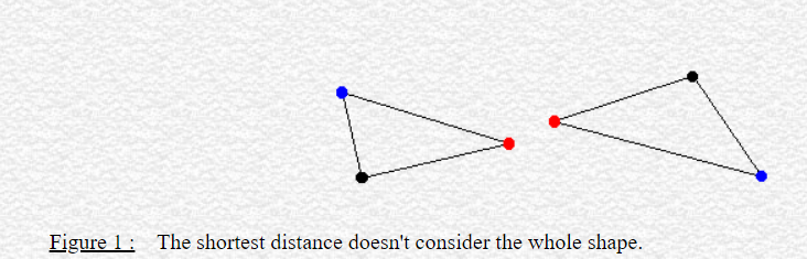
Applications: Primarily computer vision, computer graphics, digital fabrication, 3D-printing, and modeling. For example, in computer vision, it is often desirable to identify a best-candidate target relative to some initial template. In reference to the set of points within the template, the Hausdorff distance can be computed for each potential target. The target with the minimum Hausdorff distance would qualify as being the best fit, ideally being a close approximation to the template object.
Motivation: Objects are geometrically complex. There are different ways to compare objects to each other via a range of geometry processing techniques and geometric properties. Distance is often a common metric of comparison. But what type of distance should we use, which distances are favorable, and why? These are important questions.
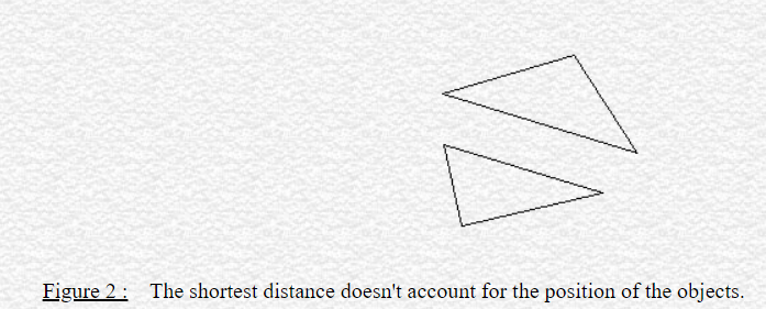
Pitfalls of using other types of distance for triangular meshes
For our research, we focus on computing the Hausdorff distance \(h\). “Hausdorff” may seem familiar to you if you know topology. There, a (topological) space is considered Hausdorff if any two elements can be separated into disjoint (open) sets. The key idea here is the separation property with respect to points.
In geometry processing, this idea is extended (in some sense) to the separation of triangle meshes. The Hausdorff distance \(h\) is fundamentally a maximum distance among desirable distances between 2 meshes. These desirable distances are minimum distances of all possible vectors resulting from points taken from the first mesh to the second mesh. But why is \(h\) significant? If \(h\) converges to zero (the smallest possible distance), then this implies that our meshes, and therefore the objects themselves, are very similar. This, like most things in math, implies within some epsilon, representing marginal change such as a slight deformation, rotation, translation, compression, or stretch. If \(h\) is large, then this implies that the two objects are dissimilar. Intuitively, this is due to a lack of ideal correspondence from triangle to triangle. In short, \(h\) serves as a means of computing the similarity between digital objects in terms of maximally separating the meshes’ points according to their minimum distances.
Tasks: To compute \(h\), we find the maximizer, the point (in the first mesh) corresponding to the computation of \(h\). This point is found via an algorithmic process called the branch and bound technique. Sparing the details, the result of applying this technique will provide a (very small) region where the minimizer is claimed to exist, after a series of triangle subdivisions and deletions. There are different ways to implement this technique. Our collective goal this week was to achieve accurate \(h\) given any two meshes. Once this is ensured, Week 2 would focus on making our code more robust (efficient/fast). This work can be simplified into three primary tasks: encoding the lower bound and upper bound of possible values of \(h\), and the subdivision method. My work focused on the lower bound, for which the other two functions are dependent.
Accomplishments: By Day 2, we started with writing pseudocode for the lower bound, using only the vertices of the first mesh and computing their distances with respect to vertices of the second mesh. This was computed per face, and the minimum was found. Although this method was correct, it didn’t account for either the edge or interior cases of a given triangle. Looping through an edge would be immediately doable, but the interior case would be more challenging. Thankfully, Dr. Sacht had us search through gptoolbox for such functionality that would account for all three cases. Once finding this function, we were able to reduce my code to two lines! The irony is although this was valid, the referenced function was basically an empty shell. The function was actually calling a C++ function that would have to compiled and linked against other libraries and due to our time constraints we decided it was best to address this issue in a future time. Ultimately, we ended up having to write from scratch once more. In searching for similar point-triangle distance algorithms, we initially found an approach using normal vectors, which would offer projective power of the former mesh vertices relative to the latter mesh. The computations were erroneous and misrepresentative. Since then, our team has been using a combinatorial plane-vector approach to find the lower bounds per vertex.
Hopefully we’ll finish soon… we’re excited for the next steps!
Isogeometric analysis (IGA) is an analysis technique that combines computer aided design (CAD) with traditional finite element analysis (FEA). It uses the same spline basis functions to construct the geometry and the solution space, which is beneficial as traditional FEA requires geometric approximation that can lead to inaccuracies [1].
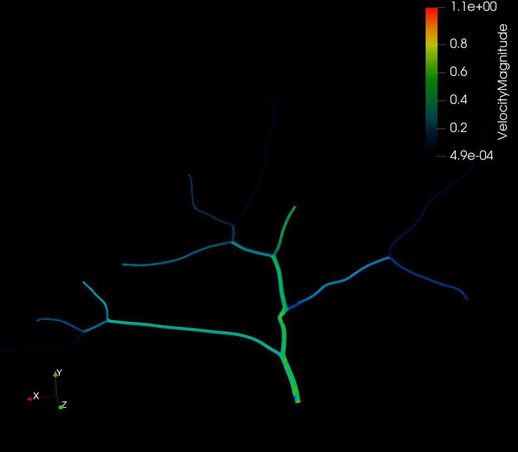
For our week 3 project, my group and I used IGA simulation software that has been developed for modelling material transport in neurons. The software solves Navier-Stokes equations to obtain the velocity field and models the transport process by reaction-diffusion-transport equations. For our purposes, we used the solver to simulate material transport in complex neurons and heat transfer processes in various geometries including a simple block model and a rod model [2].
Our project was split into two main parts: geometric modeling and analysis. For geometric modelling, we used two open source software packages (HexGen and Hex2Spline [3]) for the construction of geometries, and we then used the aforementioned IGA software for simulation purposes. I was in charge of using the IGA software to run the simulations and visualizing the results with Paraview (a visualization application).
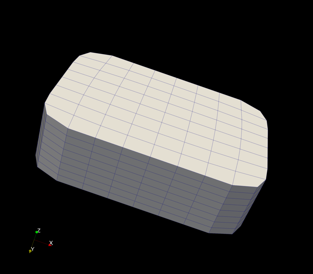
In this post, I’ll demonstrate our results using the simple model the team created and also share some of the results I got using the IGA software on some additional models.
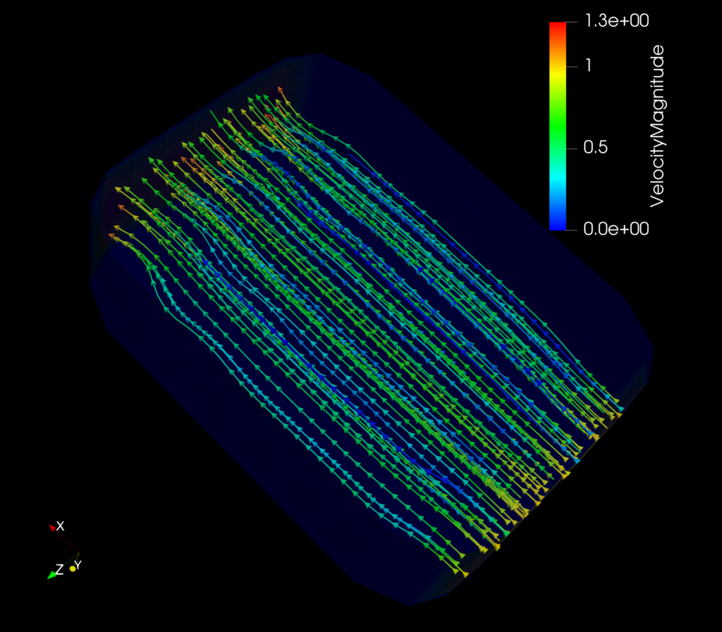
Here is the example model we used:
After the geometric modeling stage, I received 3 input files that contained the control mesh, an initial velocity field and the simulation parameters (particle concentrations, diffusion coefficient, velocities of material, etc.). These files were used as input for the IGA solver [2], which consists of four stages: spline construction, mesh partition for parallel computing, solving Navier-Stokes equations, and final transport simulation.
Due to the high computational needs of the last two stages, we set up the simulation environment at the Pittsburgh Supercomputer Center (PSC). We ran the simulation by connecting to the remote supercomputer via an ssh client. Finally, after getting the results, I was able to visualize them using Paraview.
In the above example, the color bar shows the transport velocity magnitude. I also added streamlines that show the direction of flow.
Here is an animation of our results that depicts the movement of the particles:
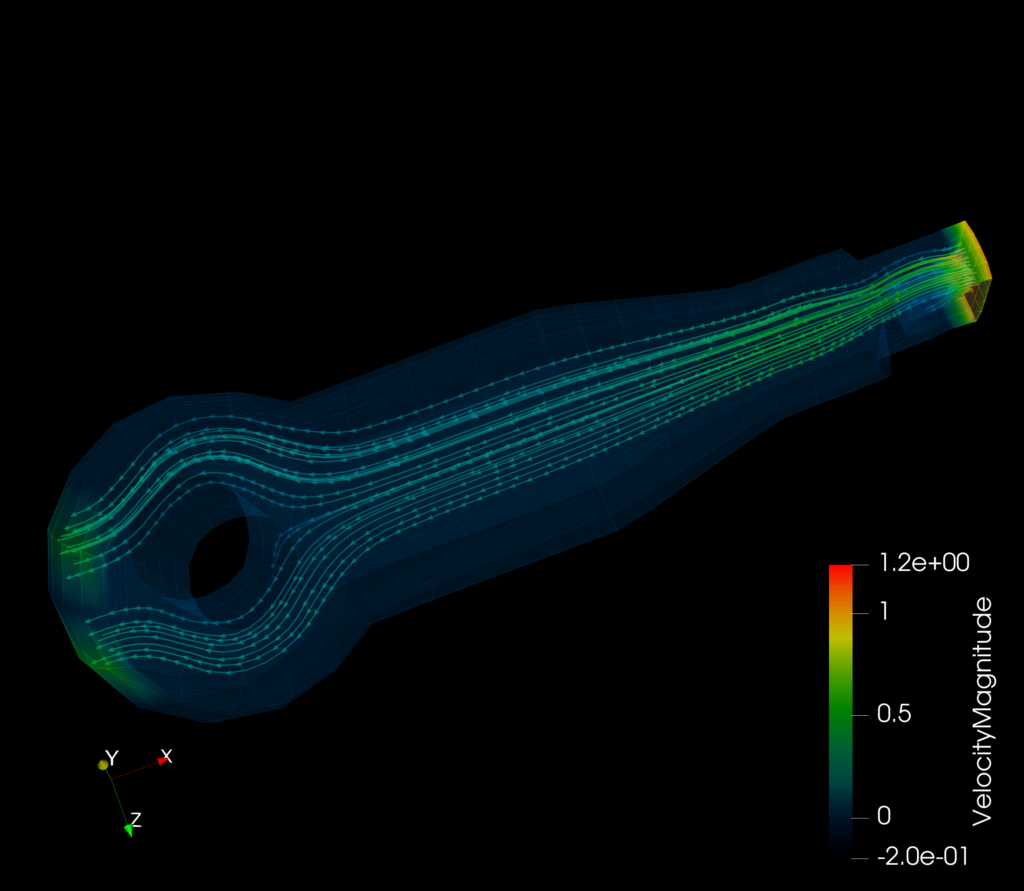
I also ran the solver on a rod model (that Angran Li, our mentor, provided):
The model shows the flow of heat through the rod as it is input from the right end of the model. Again, the colorbar represents the magnitude of the velocity of particles at that point.
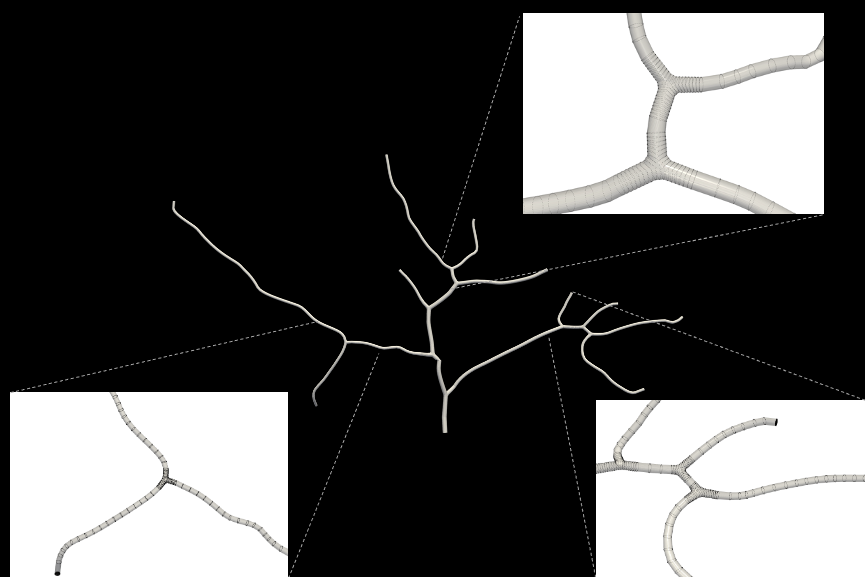
Finally, I also ran the IGA solver on a neuron model (found on NeuroMorpho.org and edited with the help of Angran).
The geometry of the neuron (visualised using Paraview)
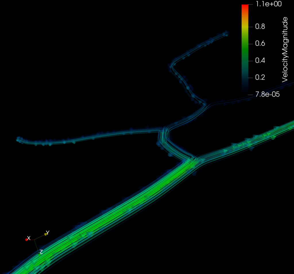
Images show results we got by running the IGA solver on the neuron geometryThe transport of material through the neuron over time
From using the remote computer to editing the neurons for our analysis, I learned a ton of new techniques during the week. I enjoyed learning about the IGA solver and its applications ranging from neuroscience to engineering. I’d like to end this post by thanking Angran his support and for bearing with me through my 1000 questions—it was a pleasure learning with you! 🙂
References:
[1] T. J. Hughes, J. A. Cottrell, Y. Bazilevs. Isogeometric analysis: CAD, finite elements, NURBS, exact geometry and mesh refinement.Computer Methods in Applied Mechanics and Engineering, 194(39-41), 4135-4195, 2005.
[2] A. Li, X. Chai, G. Yang, Y. J. Zhang. An Isogeometric Analysis Computational Platform for Material Transport Simulations in Complex Neurite Networks.Molecular & Cellular Biomechanics, 16(2):123-140, 2019. GitHub link: https://github.com/CMU-CBML/NeuronTransportIGA
[3] Y. Yu, X. Wei, A. Li, J. G. Liu, J. He, Y. J. Zhang. HexGen and Hex2Spline: Polycube-Based Hexahedral Mesh Generation and Unstructured Spline Construction for Isogeometric Analysis Framework in LS-DYNA. Springer INdAM Serie: Proceedings of INdAM Workshop “Geometric Challenges in Isogeometric Analysis”. Rome, Italy. Jan 27-31, 2020. GitHub link: https://github.com/CMU-CBML/HexGen_Hex2Spline
Written by Deniz Ozbay, Tal Rastopchin, and Alexander Rougellis
Surface Deformation and Remeshing
Representing a curved surface with a mesh of polygons can prove to be difficult because, given that meshes are discrete surfaces, there are times when small changes to the triangulation of the surface can cause big changes to the overall geometry and measured quantities (as can be seen with the example of the Schwarz Lantern). Sometimes we want to deform surfaces, and the deformation of the surface can result in a “bad” triangulation. Representing these surfaces with such deformations is done by optimizing these deformations \(\delta S\) on the given surface by solving \(\min_{\delta S} f(S + \delta S)\) where \(S\) is that given surface. When the real valued function \(f: S \rightarrow \mathbb{R}\) gives us surface area, our optimization will minimize the surface area, which is also known as mean curvature flow. Minimizing surfaces can be done with gradient descent (given a small triangle mesh) and Newton’s Method (given a large mesh). After minimizing, if the surface is determined to be “bad”, then remeshing is needed using remeshing operations such as edge flip, edge split, and edge collapse (to name a few basic operations that could be used).
Mean Curvature Flow
Given that one of the goals of this project is to optimize functions on meshes, our first task was to put together a simple implementation of mean curvature flow in MATLAB. Professor Etienne Vouga introduced mean curvature flow as a deformation of a surface that minimizes surface area. He explained that if we have a function for the surface area of a mesh, as well as the gradient, we can use an optimization method like gradient descent in order to compute the deformation induced by the mean curvature flow. After our introduction to geometry processing during the tutorial week we knew that we could use the doublarea function to write a function that returned the surface area of a mesh. However, computing the gradient of this function is tricky—what would even be the domain of the surface area function? If the doublearea function relies on computing triangle areas using the cross product, and we are summing the result over all triangles in a mesh, is the domain some sort of “collection of triangles” that we are summing over?
To answer this question, Professor Etienne Vouga pointed us to the paper “Can Mean-Curvature Flow be Modified to be Non-singular?” and explained that we could express the gradient of the surface area function as the Laplacian applied to the \(x\), \(y\), and \(z\) vertex coordinate columns. In particular, the paper explained that “informally, mean-curvature flow can be thought of as a flow that pushes a point on a surface towards the average position of its neighbors.” The paper specifically explains that when \(M\) is a two dimensional manifold, \(\Phi_t : M \rightarrow \mathbb{R}^3\) is a smooth family of immersions of the manifold \(M\), and \(g_t( \cdot, \cdot)\) is a metric induced by the immersion at time \(t\), we have that \(\Phi_t\) is a solution to the mean-curvature flow if
where \(\Delta_t\) is the Laplace-Beltrami operator defined with respect to the metric \(g_t\). If we interpret the Laplacian as a local averaging operator, this equation exactly captures the idea that mean-curvature flow is a deformation that pushes a point on a surface towards the average position of its neighbors.
For our implementation, Professor Vouga explained that instead of worrying about the metric induced by the flow we could just compute the Laplacian matrix for the first step and use it throughout the entire simulation. One thing we learned was that sometimes for computation and derivation it can be easier to look at the same function, like surface area, from a bunch of different perspectives. For example, once we knew that the gradient of the surface area was the Laplacian of the \(V\) matrix, we could compute the Hessian by reshaping the \(V\) matrix into a column vector and reshaping the Laplacian matrix into a larger block matrix with 3 copies of the Laplacian matrix along the diagonal. Computing the Hessian in this way allowed us to also try to implement a Newton’s method approach to minimize surface area.
After a lot of discussion, programming, testing, and playing around with initial conditions, we finally got our MATLAB implementation of mean curvature flow to work.
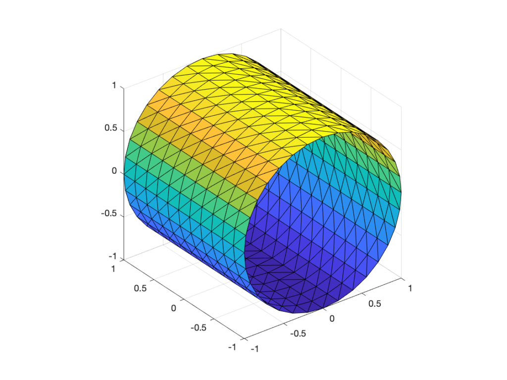
A figure displaying the open cylinder mesh used as a seed surface for the mean curvature flow.
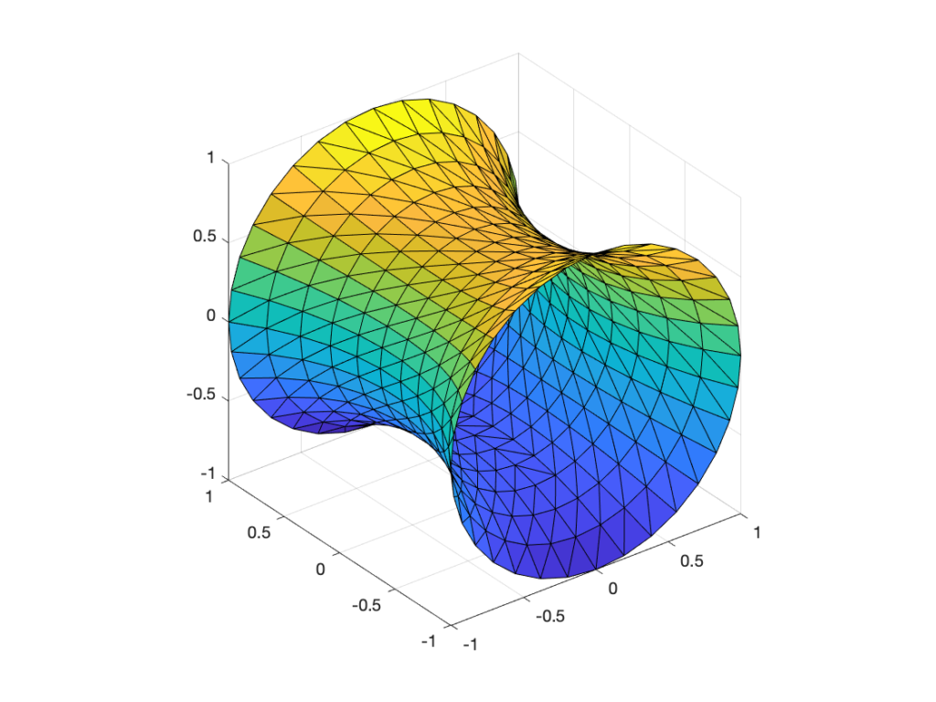
A figure displaying the catenoid mesh resulting from the mean curvature flow.
The figure on the left is a cylinder that was our initial surface and the figure on the right is the resulting minimal surface produced by the mean curvature flow. It was really cool to see the end result—the resulting minimal surfaces can be very pretty. We’re excited to learn more about optimization on surfaces as well as how remeshing could potentially improve this simulation process.
Current and Future Work
Currently, we are working on implementing Newton’s method and the gradient descent method in the same program as remeshing. Our algorithm runs Newton’s method as long as it decreases the surface area. If a Newton step does not decrease the surface area, the algorithm then switches to the gradient descent method. Then it remeshes the triangles using edge flipping to obtain a Delaunay triangulation. To build this code, we made use of numerous different structures, like an edge face matrix, edge vertex matrix and a vertex face matrix. Then, we were able to implement the edge flipping condition. At this step we first find the neighboring two faces of the edge we check to flip. We check if the angles at the third vertices of the corresponding two faces is bigger than \(\pi\) radians, and if so, the edge is flipped to get the remeshing closer to a Delaunay triangulation. This allows us to optimize the surface and do the remeshing at the same time, which we think is very cool!
While implementing our algorithm, we did lots of debugging and got some funny shapes. Of course, one of the best parts about trying to make the code work was working together as a team. We had a lot of fun trying to decipher what went wrong when we got surfaces compressing to lines then to funny looking disks. Our next step is to work on coming up with algorithms for edge split and edge collapse, so we can fully implement remeshing on the shape. We are really excited to see what the final product will look like, to try lots of cool surfaces and see what the optimized remeshing for each will be!
By: Natasha Diederen, Joana Portmann, Lucas Valença
These past two weeks, we have been working with Paul Kry to extend Jos Stam’s work on stable, incompressible fluid flow simulation. Stam’s paper Flows on Surfaces of Arbitrary Topology implements his stable fluid algorithm over patches of Catmull-Clark subdivision surfaces. These surfaces are ideal since they are smooth, can have arbitrary topologies, and have a quad patch parameterisation. However, Catmull-Clark subdivision surfaces are a quite specific class of surface, so we wanted to explore whether a similar algorithm could be implemented on triangle meshes to avoid the subdivision requirement.
Understanding basics of fluid simulation algorithms
We spent the first week of our project coming to terms with the different components of fluid flow simulation, which is based on solving the incompressible Navier-Stokes equation for velocities (1) and a similar advection-diffusion equation for densities (2) \[ \frac{\partial \mathbf{u}}{\partial t} = \mathbf{P} { -(\mathbf{u} \cdot \nabla)\mathbf{u} + \nu \nabla^2 \mathbf{u} + \mathbf{f} }, \quad (1)\] \[\frac{\partial \rho}{\partial t} = -(\mathbf{u} \cdot \nabla)\rho + \kappa \nabla^2 \rho + S, \quad (2)\] where \( \mathbf{u}\) is the velocity vector, \(t\) is time, \(\mathbf{P}\) is the projection operator, \( \nu\) is the viscosity coefficient, \(\mathbf{f}\) are external sources, \( \rho\) is the density scalar, \( \kappa\) is the diffusion coefficient, and \( S \) are the external sources. In the above equations, the Laplacian (often denoted \( \Delta\)) is written as \( \nabla^2\), as is usually done in works from the fluids community.
In his paper, Stam uses a splitting technique to deal with each term on its own. The algorithm carries out the following steps twice: first for the velocities and then for the densities (with no “project” step required for the latter). \[ \mathbf{u_0} {\underset{\overbrace{\text{add force}}^\text{ }}{\Rightarrow}} \mathbf{u_1} {\underset{\overbrace{\text{diffuse}}^\text{ }}{\Rightarrow}} \mathbf{u_2} {\underset{\overbrace{\text{advect}}^\text{ }}{\Rightarrow}} \mathbf{u_3} {\underset{\overbrace{\text{project}}^\text{ }}{\Rightarrow}} \mathbf{u_4} \]
We start by adding any forces or sources we require. In the vector case, we can add acceleration forces such as gravity (which changes the velocities) or directly add velocity sources with a fixed location, direction, and intensity. In the scalar case, we add density sources that directly affect other quantities.
Single density source pouring down with gravity over an initially zero velocity field
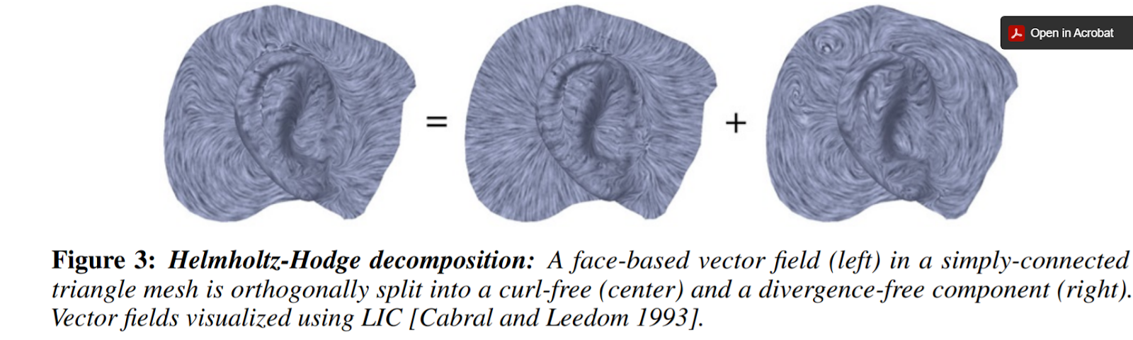
Densities and velocities are moved from a high to low concentration in the diffusion step, then moved along the vector field in the advection step. The final projection step ensures incompressible flow (i.e., that mass is conserved), using a Helmholtz-Hodge decomposition to force a divergence-free vector field. We will not go into much more detail on Stam’s original Stable Fluids solver. Dan Piponi’s Papers We Lovepresentation gives a very comprehensive introduction for those interested in learning more.
To better understand the square grid fluids solver, we implemented a MATLAB version of the C algorithm described in Stam’s paper Real-Time Fluid Dynamics for Games. In terms of implementation, since we were coding in MATLAB, we did not use the Gauss-Seidel algorithm (like Stam did) to solve the minimisation problems. Instead, we solved our own quadratic formulations directly. Although some of our methods differed from the original, the overall structure of the code remained the same.
Full simulation results over a square grid can be seen below.
Generalising to triangle meshes
After a week, we understood the stable fluid algorithm well enough to extend it to triangle meshes. Stam’s paper for triangle meshes adapted the algorithm above from square grids to patches of a Catmull-Clark subdivided mesh, with the simulation boundary conditions at the edges of the parametric surfaces. We, on the other hand, wanted a method that would work over any triangular mesh, as long as such mesh, as a whole, is manifold without boundary. Moreover, we wished to do so by working directly with the triangles in the mesh without relying on subdivision surfaces for parameterisation. The main difference between our method and Stam’s was the need to deal with the varying angles between adjacent faces and their effect on advection, diffusion, and overall interpolation. In addition, since we’re working with manifolds without boundaries, we did not need to deal with boundary conditions (like in our 2D implementation). Furthermore, we had to choose between storing both vector and scalar quantities at the barycentre of each face or at each vertex. For simplicity, we chose the former.
What follows is a detailed explanation of how we implemented the three main steps of the fluid system: diffusion, advection and projection.
Diffusion
To diffuse quantities, we solved the equation\[ \dot{\mathbf{u}} = \nu \nabla^2 \mathbf{u},\] which can be discretised using the backwards Euler method for stability as follows \[ (\mathbf{I}-\Delta t \nu \nabla^2)\mathbf{u_2} = \mathbf{u_1}.\] Here, \( \mathbf{I} \) is the identity matrix and \( \mathbf{u_1}, \ \mathbf{u_2} \) are the respective original and final quantities for that iteration step, and can be either densities or vectors.
Surprisingly, this was far easier to solve for a triangle mesh than a grid due to the lack of boundary constraints. However, we needed to create our own Laplacian operators. They were used to deal with the transfer of density and velocity information from the barycentre of the current triangle to its three adjacent triangles. The first Laplacian we created was a linear operator that worked on vectors. For each face, before combining that face’s and its neighbours’ vectors with Laplacian weighting, it locally rotated the vectors lying on each of the face’s neighbouring faces. This way, the adjacent faces lay on the same plane as the central one. The rotated vectors were further weighted according to edge length (instead of area weighting) since we thought this would best represent flux across the boundary. The other Laplacian was a similar operator, but it worked on scalars instead of vectors. Thus, it involved weighting but not rotating the values at the barycentres (since they were scalars).
Diffusion of scalars over a flattened icosahedron
Advection
Advection was the most involved part of our code. To ensure the system’s stability, we implemented a linear backtrace method akin to the one in Stam’s Stable Fluids paper. Our approach considered densities and velocities as quantities currently stored at barycentres. It first looked at the current velocity at a chosen face then walked along the geodesic in the opposite direction (i.e., back in time). This allowed us to work out which location on the mesh we started at so that we would arrive at the current face one time-step later. This is analogous to Stam’s 2D walking over a square grid, interpolating quantities at the grid centres, but with a caveat. To walk the geodesics, we first had to use barycentric coordinates to work out the intersections with edges. Each time we crossed an edge, we rotated the walk direction vector from the current face to the next, making it as if we were walking along a plane. At the end of the geodesic, we obtain the previous position for the quantity on our current position. We then carried out a linear interpolation using barycentric coordinates and pre-interpolated vertex data. The result determined the previous value for the quantity in question. This quantity was then transported back to the current position. Vector quantities were also projected back onto the face plane at the end to account for any numerical inaccuracies that may have occurred.
Advection of a density blob over an icosahedron following gravity
Our advection code initially involved walking a geodesic for each mesh face, which is not computationally efficient in MATLAB. Thus, it accounted for the majority of the runtime of our code. The function was then mexed to C++, and the application now runs in real-time for moderately-sized meshes.
Projection
So far, we have not guaranteed that diffusion and advection will result in incompressible flow. That is, the amount of fluid flowing into a point is the same as the amount of fluid flowing out. Hence, we need some way of creating such a field. According to the Helmholtz-Hodge decomposition, any vector field can be decomposed into curl-free and divergence-free fields, \[ \mathbf{w} = \mathbf{u} + \nabla q, \] where \( \mathbf{w}\) is the velocity field, \( \mathbf{u} \) is the divergence-free component, and \( \nabla q\) is the curl-free component.
A solution (for \(q\)) is implicitly found by solving a Poisson equation of the form \[ \nabla \cdot \mathbf{w} = \nabla^2 q\] where we used the cotangent Laplacian in gptoolbox for \(\nabla^2 q\). Subtracting the solution from the original vector field gives us the projection operator \( \mathbf{P}\) to find the divergence free component \( \mathbf{u} \) \[\mathbf{u} = \mathbf{Pw}=\mathbf{w}-\nabla q. \]
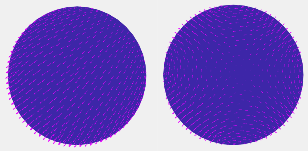
A uniform vector field before (left) and after (right) projection
This method works really nicely for our choice of having vector quantities stored at the faces. The pressures we get will be at the vertices. The gradients of those pressures are naturally computed at faces to alter the velocities to give an incompressible field. The only challenge is that the Laplacian is not full rank, so we need to regularise it by a small amount.
Future work
We would like to implement an alternative advection method, possibly more complicated. This method would involve interpolating vertex data and walking along mesh edges, rather than storing all our data in faces and walking geodesics crossing edges. This could possibly avoid extra blurring, which might be introduced by our current implementation. This occurs because we must first interpolate the data at the neighbouring barycenters to the vertices. This data is then used to do a second interpolation back to the barycentric coordinate the geodesic ends at.
For diffusion, although our method worked, there were a few things that could be improved upon. Mainly, diffusion did not look isotropic in cases with very thin triangles, which could be improved by an alternative to our current weighting of the Laplacian operator. Alternatively, we could use a more standard Laplacian operator if we stored quantities at the vertices instead of barycenters. This would result in more uniform diffusion at the expense of a more complicated advection algorithm.
Example of non-isotropic diffusion over a flattened torus
Conclusion
Final results
We would like to give a thousand thanks to Paul Kry for his mentorship. As a first foray into fluid simulations, this started as a very daunting project for us. Still, Paul smoothly led us through it by having dozens of very patient hours of Zoom calls, where we learned a lot about maths and coding (and biking in the rain). His enthusiasm for this project was infectious and is what enabled us to get everything working in such a short period. Still, even though we managed to get a good start on extending Stam’s methods to more general triangle meshes, there is a lot more work to do. Further extensions would focus on the robustness and speed of our algorithms, separation of face and vertex data, and incorporation of more components such as heat data or rotation forces. If anyone would like to view our work and play around with the simulations, here is the link to our GitHub repository. If anybody has any interesting suggestions about other possibilities to move forward, please feel free to reach out to us! 😉
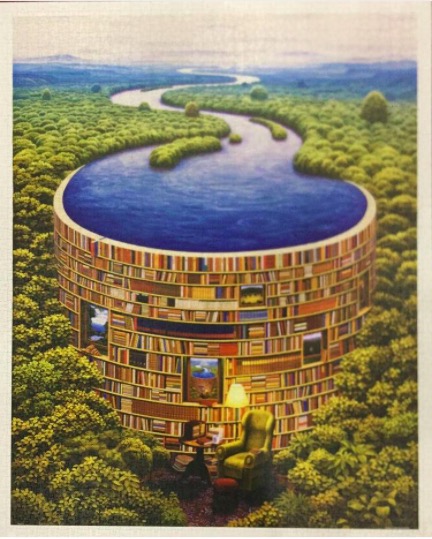
Disclaimer: If you are looking for a technical and mathematical post, this is not the one for you! But if you share a passion for jigsaw as I do, feel free to scroll through and enjoy my 2000-piece jigsaw puzzle below.
“Click” went the sound of the final piece of the 2000-piece puzzle. 4 days, 18 cumulative hours spent, and the result lied magnificently in front of my eyes: a beautiful cozy library underneath a never-ending river—another one goes to the collection.
My proud 2000-piece jigsaw puzzle
Puzzles are my refuge, a much-valued pastime. As I painstakingly classified, searched for pieces, and watched the puzzle slowly come into place, my thoughts ran wild: I marveled at the perfect cut coming from my Ravensburger puzzle set, wondering how a laser-cut could be so clean. That’s why when I came to MIT SGI this summer, my eyes were immediately caught on the project “Optimal Interlocking Parts via Implicit Shape Optimization” by Professor David Levin.
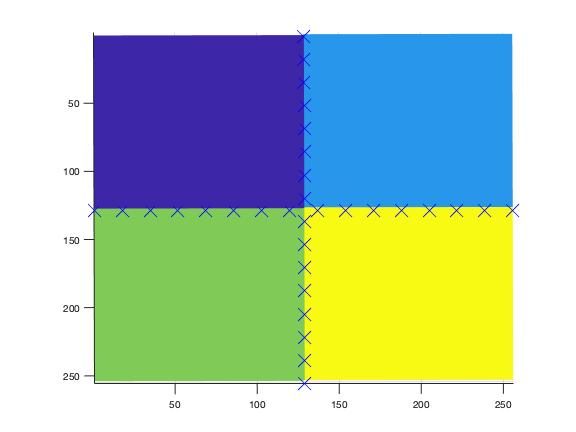
In the project, I learned about the polygonizer technique, with which we tried to cut the puzzle into pieces based on known clusters. The process involves two steps:
Firstly, we found points on the cut lines.
Secondly, we connected the points above to create shapes for the puzzle pieces.
Simple illustration of polygonizer technique (step 1)
Due to the time constraint, I was not able to fully finish implementing this technique, but the project gave me hindsight on how puzzles are created with such precision and weirdness in piece shapes (recalling the crazy and infamous Krypt puzzle of Ravensburger). Like the feeling of finishing a giant jigsaw puzzle, the excitement of having my code run smoothly on a test image is equivalently comparable!
The SGI research program has been structured in a novel way in which each project lasts for one or two weeks only. This gives Fellows the opportunity to work with multiple mentors and in different areas of Geometry Processing. A lot of SGI fellows, including me, had wondered how we would be able to finish the projects in such a short period of time. After two weeks, as I pause my first research project at SGI, I am reminded of Professor Solomon’s remark that a surprising amount of work can be done within 1/2 weeks when guided by an expert mentor.
In this post, I have shared the work I have done under the mentorship of Prof. David Levin over the last two weeks.
Optimal Interlocking Parts via Implicit Shape Optimizations
In this project, we explored how to automatically design jigsaw puzzles such that all puzzle pieces are as close to a given input shape \(I\) as possible, while still satisfying the requirement of interlocking.
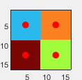
Lloyd relaxation with Shape Matching metric
As the first step, we needed a rough division of the domain into regions corresponding to puzzle pieces. For this initial division we used Lloyd’s relaxation as it ensured that the pieces would interlock. To create regions similar to the input shape, we employed a new distance metric. This metric is based on shape matching.
Shape Matching metric:
The input shape \(I\) is represented as a collection of points \(V\) on its boundary and is assumed to be of unit size and centered at the origin. Consider a pixel \(p\) and a site \(x\). First the input shape is translated to \(x\) ( \(V \rightarrow V’\)). The value of scaling factor \(s\) that minimizes the distance between \(p\) and the closest point \(V’_i\) on the boundary of the input shape gives us the shape matching metric. \[s^* = \text{arg min} \frac {1} {2}(dist(p, sV’))\]
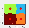
Results of Lloyd’s relaxation with shape matching in a 16X16 domain for Input Shapes: Square and a Puzzle piece respectively.
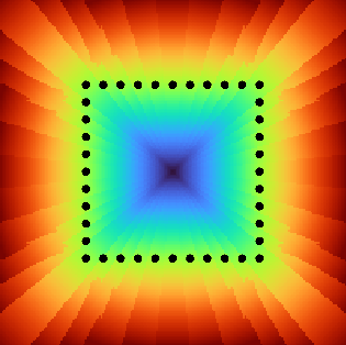
Pre computing maps
The straightforward implementation for Lloyd’s relaxation that I had been using was iterative and therefore very slow. In fact, testing the algorithm for larger domains or complicated shapes that needed dense sampling of boundary points was infeasible. Therefore, optimizing the algorithm was an immediate requirement. I realized that relative to the site \(x\), the distances would vary around it in exactly the same way. So, computing the distance between each pixel and each site separately during each iteration of Lloyd’s relaxation was redundant and could be avoided by pre-computing a distance map for the given object before starting Lloyd’s relaxation.
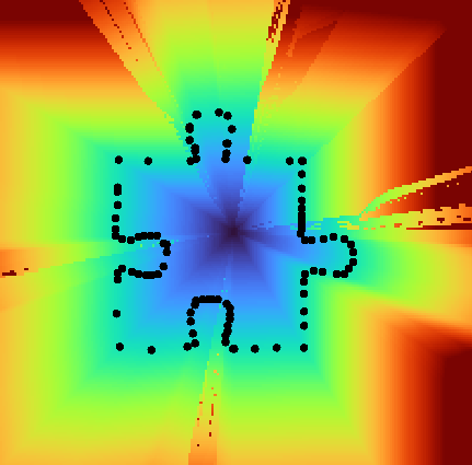
200×200 maps for square input shape and puzzle piece. The input shape has been scaled and overlaid on top of the map for clarity.
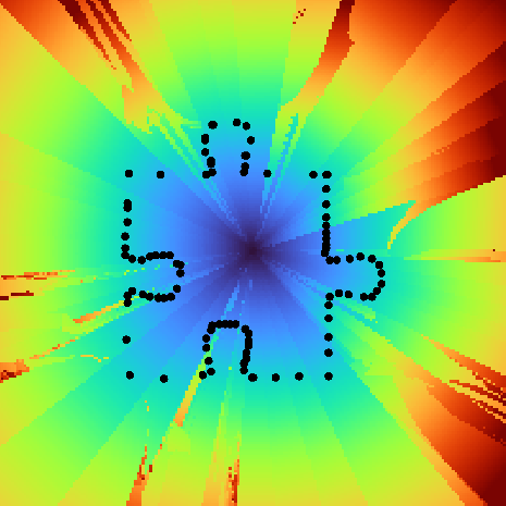
Enhancing the shape matching metric
In addition to speeding up the algorithm, the distance maps also helped in determining the next step. As can be seen from the figures above, the maps weren’t smooth. These jumps in distance fields occurred because the shape matching metric worked on a set of discrete points. Optimizing the scaling factor for minimizing distance to the closest edge instead of closest point resolved this.
200×200 Map with enhanced Shape Matching metric input shape of a puzzle piece.
Shaping the puzzle pieces (In progress)
The initial regions are obtained from Lloyd’s algorithm with the shape matching metric need to be refined so that the final puzzle pieces are highly similar to the input shape \(I\).
I am currently exploring the use of point set registration methods to find the best transformations on the input shape so that it fits the initial regions. These transformations could then be used to inform the next iteration of Lloyd’s algorithm to refine the regions. This process can be repeated until the region stops changing, giving us our final puzzle pieces.
I have thoroughly enjoyed working on this project, and I am looking forward to the next project I would be working on!
What does it mean for a shape to be complex? We can imagine two shapes and decide which seems to be more complex, but is our perception based on concrete measures? The goal of this project is to develop a rigorous and comprehensive mathematical foundation for shape complexity. Our mentor Kathryn Leonard has conducted previous work on this topic, categorizing and analyzing different complexity measures. The categories include Skeleton Features, Moment Features, Coverage Features, Boundary Features, and Global Features. This week we focused primarily on two complexity measures from the Boundary Features. We tested these measures on an established database of shapes as well as producing some shapes of our own to see which aspects of complexity they measure and if they match our intuition.
Measures
Boundary
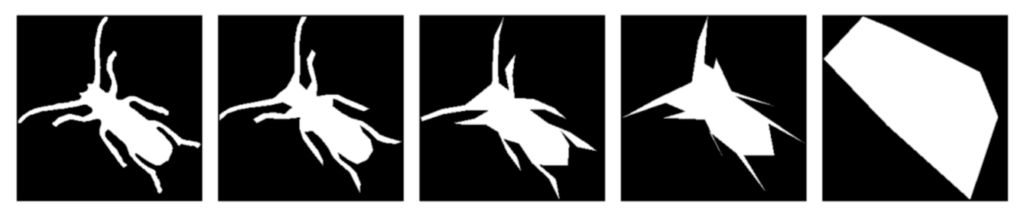
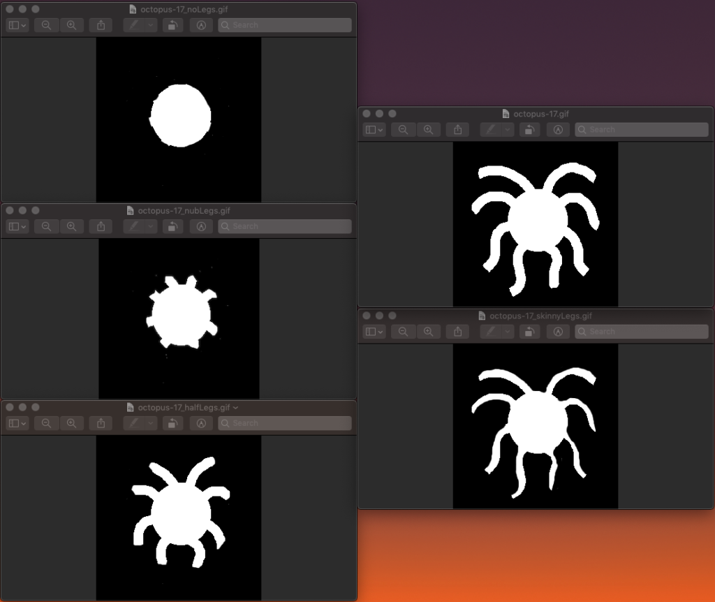
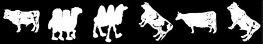
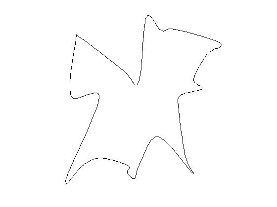
The first measure of complexity we considered was related to the boundary of the figure. To understand the measure, we first need to understand down-sampling. This is the process of lowering the number of vertices used to create the shape, and using a linear approximation to re-create the boundary. A total of five iterations were performed for each figure, typically leading to a largely convex shape.
Downsampled image with 500, 100, 50, 25, and 8 vertices.
The measure we considered was the ratio between the length of the downsampled boundary and that of the original boundary. In theory, downsampling would significantly change the boundary length of a complex shape. Thus, ratio values close to 0 are considered complex and values close to 1 are considered simple (that is, the downsampled length closely matches the original).
The boundary measure was tested on images which had been hand-edited to create a clear progression of complexity.
For example, the boundary measure created a ranking that nearly matched our intuition, besides switching the regular octopus and the octopus with skinny legs. For all other hand-edited progressions, the boundary measure exactly matched our intuition.
See Appendix 3 in the attached spreadsheet for the full boundary data.
Curvature
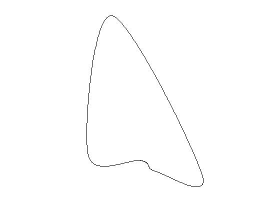
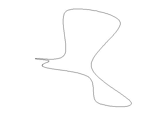
The second measure of complexity we considered was curvature. We calculate a normalized, ten bin histogram of the distribution of curvature values at each point of the shape boundary for a given shape and rank the complexity based on the value of the first bin, which was shown in user studies to be highly correlated with user rankings. Higher numbers generated from this measure indicate greater complexity.
One thing this measure emphasizes is sharp corners. At these points the curvature is very high, having a large impact on the overall value.
0.040800
0.042084
0.048096
Adding sharp bends increases complexity as measured by curvature
User Ranking
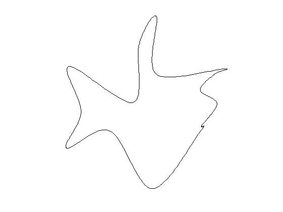
To see how these measurements compared to our conception of complexity, we looked at previously created images and ranked them as a group according to our notion of complexity. One such subset of images was a group of eight unrelated figures, shown below.
We then used the two measures to create an automated ranking.
The octopus had the lowest boundary length value, and thus the highest complexity ranking according to this measure. Much of the original figure’s perimeter is contained in the tentacles, which are smoothed out during the downsampling. This leads to a large difference in boundary lengths, meaning a more complex ranking.
As previously mentioned, the curvature measure emphasizes sharp corners. This is why the curvature measure ranks the stingray and flower higher than the boundary measure does.
To evaluate how well the resulting ranking matched with our own ordering, we used three similarity measures shown below.
Measure
Similarity Value
Avg. Distance
Normalized Dist
Boundary Length
0.3750
1.00
0.12500
Curvature
0.2500
0.75
0.09375
The first measure we used to compare the user and automated rankings was the ratio of the number of images with matching rank to the total number of images. We called this ratio the similarity value. For example, the user rankings and curvature rankings both placed ‘lizzard-9’ at #1 and ‘Glas-9’ at #6. Thus, the similarity value for the curvature measure was 2/8, or 0.25.
The second similarity measure we used was the average distance, the ratio of the sum of the differences in rank number for each image to the total number of images. This was included to consider how much the ranking of each image differed.
The third similarity measure was the normalized distance, the ratio of the average distance to the total number of images. This was included to account for differences in sample sizes.
The rankings of the group of eight images did differ from our ordering, but on average each shape was off by less than one rank.
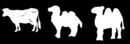
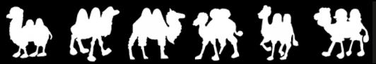
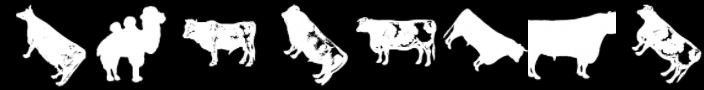
Camel & Cattle
Now that we better understand each measurement, we tested them on a database of thirty-eight images of camels and cattle. As in the first example, we ranked the images in order of perceived complexity, and then generated an ordering from the boundary length and curvature measures.
Measure
Similarity Value
Avg. Distance
Normalized Dist
Boundary Length
0
10.31578
0.27146
Curvature
0.02631
8.68421
0.22853
This ranking was less accurate, but still had a clear similarity. We did see however similar groups of values in the boundary length, and ties within the curvature and to deal with this we ran k-mediods clustering on these bins of measures individually.
See Appendix 1 for the full data on the Camel-Cattle Rankings
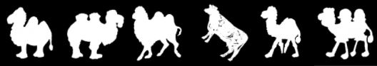
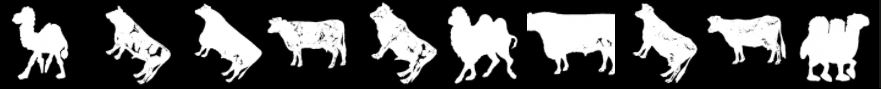
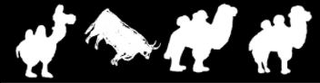
K-mediods clustering is an algorithm that puts into groups or clusters pieces of data, in an attempt to minimize the distance (in this case Euclidean distance) between the points within each cluster to minimize the total of Euclidean distances summed over the distance within each cluster. For the curvature measure we got the following clusters. (Note that the boundary length and curvature measures ignore any ‘noise’ within the boundary of the image. Thus, the spots on the cows were not considered.)
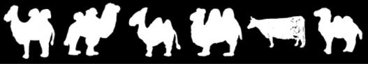
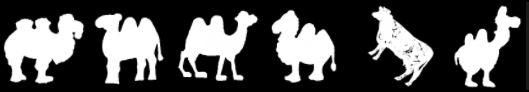
This showing what the curvature measure considers the most similar shapes, and for the boundary length measure getting the following clusters:
In order to see how well the two measures did in combination, we used both quantities in a clustering algorithm to produce groupings of similar images. The resulting clusters grouped simple shapes with simple shapes, and more complex shapes with more complex shapes.
See Appendix 2 in the attached spreadsheet for the full clusters as well as their distances on the Camel-Cattle.
Polylines
To test our measures on a clear progression of complexity, we decided to make our own shapes. Using a Catmull-Rom interpolation of a set of random points (thanks day 3 of tutorial week!), we produced a large data set of smooth shapes. Generally, intuition says that the more points used in the interpolation, the more complex the resulting shape. Our measures both reflected that pattern.
N = 5
N = 10
N = 15
N = 25
C: 0.022044 B: 1.0044
C: 0.034068 B: 0.98265
C: 0.066132 B: 0.93492
C: 0.08016 B: 0.91145
See Appendix 4 in the attached spreadsheet for the full ranking data of the measures on the Polylines.
We calculated these measures on our database of over 150 shapes, each generated from five, ten, fifteen, or twenty-five points. Using these results, a clustering algorithm was able to roughly distinguish between these four groups. It groups 98.0% of the fives together, 78.7% of tens, 62.5% of fifteens, and 85.2% of twenty-fives. We also note that both complexity measures identify these shapes as much simpler than the other shapes in our database, even with the higher point orders. This is likely because of how smooth the lines are. This reveals an opportunity for future improvement in these measures, since intuition would rank a simple shape from the database (like the horseshoe) as simpler than the figure in the N = 25 column above.
See Appendix 5 in the attached spreadsheet for the clustering data of the polylines.
Noisy Circles
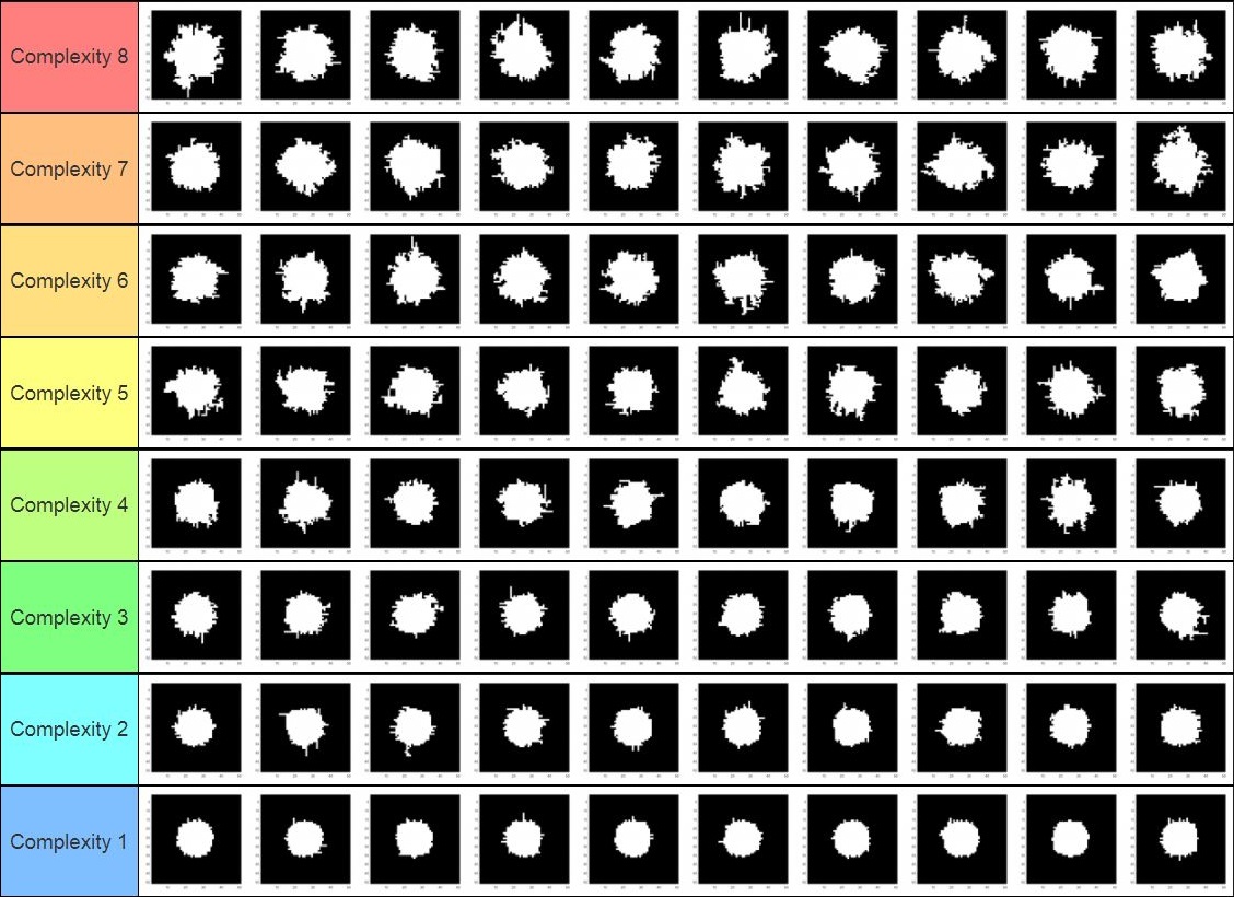
In order to test the measures on a clear progression of complexity that progressed the noise of the shape (small protrusions) rather than large protrusions or changes like in the Polylines we created we created a shape making program that started with a circle, something that both our intuition ad the constructive model of complexity put forth as the simplest shape. We then added noise to the circle by running a pseudo-random walk on each point on the boundary of the circle where we added a point for each step of the walk. The walk went in a random cardinal direction, a random number of steps for each point on the boundary, we then theorized that we would be able to add levels of complexity on average by increasing the number of propagations, eg: the number of times that the circle underwent every point taking a random walk. This has the additional benefit that like the polylines allows us to measure complexity on average levels which would give us a better comparison to see if our measures are reasonable.
To test this we ran eight levels of complexity with ten shapes per level. The shapes as well as what propagation, and thus complexity level each one is is shown in the first figure.
In order to give a partial test to see if our hypothesis that generally the more propagations are run the more complex the shape is we tested it against our human intuition of complexity, and ranked the shapes according to how complex they seemed to human intuition.
Comparing the two we get the following table:
Similarity Percentage
Distance
58.75%
0.425
At first glance looking at the similarity percentage, that is how many of the shapes are placed by human intuition into the same complexity level as the number of perturbations, and we see that only 59% of the shapes are placed into the same level, however, looking at the distance tells us a different story. We see from the small distance value, that our similarity percentage is lower than we would like because swaps between one level and another are rather common which means that the general relation of propagations to complexity is what we desire, thus comparing distance to the original seems to be a promising measure of how accurate the propagations to complexity are. As this distance function implies that on average the complexities are in the correct level and are only moved half a level from the number of propagations done. Thus as our general hypothesis is true that the number of propagations correlates to the complexity we can look at the automatic measure of propagations rather than user intuition for comparing this data to the curvature and boundary measures.
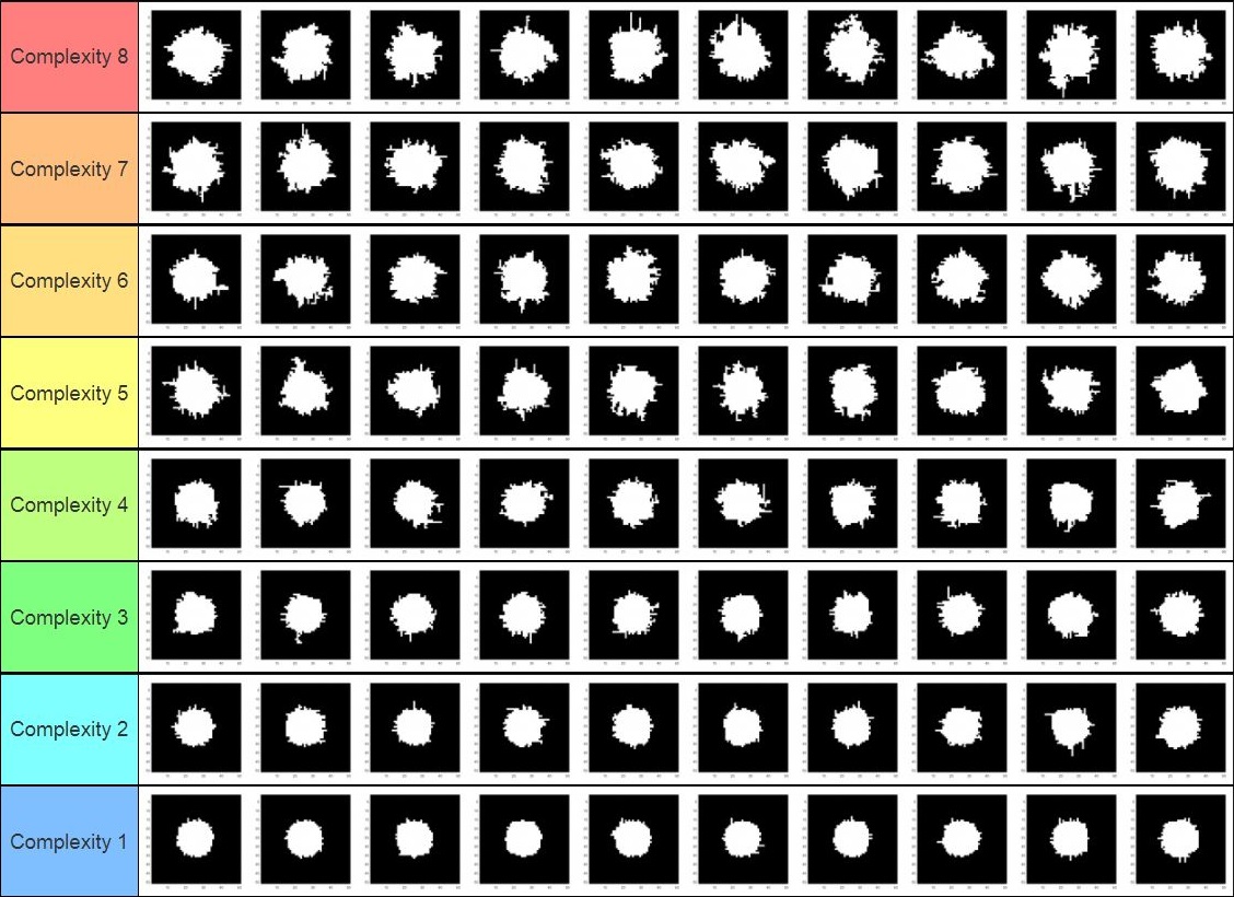
Now that we have seen this let us look at how the curvature measure ranks the shapes. In the bottom left figure:
Similarity Percentage
Distance
0.3%
1.2625
We see from the similarity, that it is less similar to the propagations, than the intuition and thus is less accurate to our intuition than the number of propagations are, however it again does not have a large distance, in fact when taking into account the distance between the the intuition and the propagation we get that the distance range between intuition and the curvature measure ranking is in the range of 0.8375-1.6875, which is not too large of a change, and shows that the curvature measure is a reasonable measure insofar that it gives us the correlation that we are looking for generally, however as we can see looking at the ranking itself in the figure it is not entirely accurate.
See Appendix 6 in the attached spreadsheet for the full ranking data for the not-circles.
We now look at the other main measure that we use the boundary length measure to see the ranking that it produces. In the bottom right figure:
Similarity Percentage
Distance
0.375%
0.8625
From this data we see that in comparison to the curvature we have both a higher similarity and a lower distance. From the low distance we see that in general only small shifts between what levels things should be placed upon occur, confirmed by the difference between the boundary length measure and our intuition being in the range of 0.4375-1.2875, this shows that for looking of noise of this nature that the boundary length measure is better than the curvature measure as it keeps the general relationship and does so with much less error, thus showing a strong reason to use the boundary length measure as a way to classify the complexity of shapes differing in the amount of noise that they have.
See Appendix 6 in the attached spreadsheet for the full ranking data.
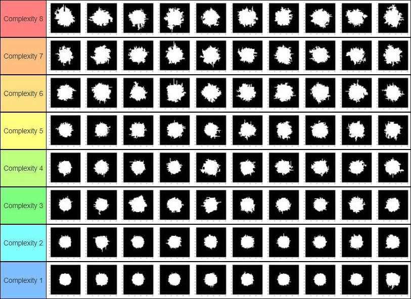
Lastly, to see whether or not these levels are somewhat arbitrary and whether there is an even gap between levels, we use k-medoids clustering on eight clusters to see how it is clustered using both the boundary length and curvature measures together. From this we get extremely interesting results, in that they say “No! There are not even gaps” we see this from the range in sizes of the clusters that occur ranging from 1 to 27, thus we see that the propagations do not create even clusters but rather bursts of complexity. This is however to be expected, the levels are simply the number of propagations that occur and we forced the earlier rankings into using the same number on each level, and thus this does not defeat that on average each level has more complexity, we also need to consider that there are some differences due to using these measures for clustering from how human intuition would cluster them. We now from seeing the lowest number of clusters have a strange result, one of the clusters has only one element in it, , and while this presents an initial puzzle after analysis it shows to have a good reason the circle like element by itself is almost a perfect (pixel) circle, thus it is placed by itself as its own level of a “zero” complexity. That many levels of propagations exist within one cluster is also similarly explained to clusters of different sizes, that is when we looked at our previous data small changes in distance were common and thus in clustering instead of small distances, where small shifts occur we instead have them in the same group.
See Appendix 7 in the attached spreadsheet for the full clusters as well as distances of the noisy circles.
Putting it all Together
Lastly we clustered everything in order to get a sense of the various complexities and how our measures would group all of the different main categories of shapes that we looked at, those being the camel-cattle, the polylines and the not circles. We put them into eight clusters in order to attempt to put them into the same category levels of complexity as were arbitrarily created by the not shape propagations. From this we got somewhat unexpected results, those being that while the camel-cattle were grouped together with the not circles, as well as with how their complexities would expect them to be grouped based on earlier clusterings, the polylines were in clusters by themselves. We then have to expand upon this clustering in order to try to explain it. The clusters of camel-cattle as well as not circles were four of the eight clusters, inside of these clusters we had on average the higher number of propagation on not circles grouped together with the camel-cattle that were given higher ranked complexity values, and vise-versa with lower propagation and lower ranked complexity. The other four clusters were the polyline data, and the reason for this is that as we can see the polylines are given by the curvature ad boundary length measures to have much less complexity and as such are in a group, well groups of their own having much less complexity than the camel-cattle as well as the not circles, and thus by our measures they are clustered separately. This is interesting especially as one of our not circles is almost just a perfect (pixel) circle, we then want to somewhat explain why this is more complex than the polylines, and the answer that we see for this is that the polylines are much smoother, while the pixel circle is still made out of these large pixels and thus is much sharper, it is thus left as a somewhat open question if this would be true for larger starting not circles.
See Appendix 8 in the attached spreadsheet for the full clusters as well as the distances of all the shapes.
Conclusion
From our tests and calculations, we conclude that our intuition of shape complexity is measurable, at least according to some respects, we saw that curvature was a good measure of how many sharp edges a shape has, and length was a measure of the noise and somewhat of the protrusions on a shape. The specific measurements of boundary length and curvature both give good estimations of complexity, giving the general relation between our intuitive understanding, while measuring in general different properties of shapes. However, we only did this research for one week and thus it feels necessary to say what would be done to continue on this research, the ways that we would continue the research is in three main facets. Firstly we would like to use more measures other than just the boundary length and curvature measures, in order to both see if there are other more effective general measures of complexity and in order for us to see if other measures are better able in particular at looking at different areas of complexity. From looking at more measures we can also increase what we consider in our k-medoids. The second thing that we would do is to compare and rank more of the shapes based on the intuition of more people, because of the subjective nature of doing this intuitive ranking. This would allow us to better with more data on subjective ranking see how accurate our complexity measurements are. On this same subject the third area we would do more research on would be to increase the number of shapes that we are looking at specifically the number of not circles, and polylines as they are randomly generated and thus only on average increase in complexity and thus with the more shapes we have of them the clearer we would see the differences in complexity between the number of points and the propagations.
Acknowledgements
We would like to express great appreciation for our mentor Kathryn Leonard, who generously devoted time and guidance during this project. We would also like to thank our TA Dena Bazazian, who provided feedback and encouragement throughout the week.