Authors: Bryce Van Ross, Talant Talipov, Deniz Ozbay
The SGI project titled Robust computation of the Hausdorff distance between triangle meshes originally was planned for a 2 week duration, and due to common interest in continuing, was extended to 3 weeks. This research was led by mentor Dr. Leonardo Sacht of the Department of Mathematics of the Federal University of Santa Catarina (UFSC), Brazil. Accompanying support was TA Erik Amezquita, and the project team consisted of SGI fellows, math (under)graduate students, Deniz Ozbay, Talant Talipov, and Bryce Van Ross. Here is an introduction to the idea of our project. The following is a summary of our research and our experiences, regarding computation of the Hausdorff distance.
Definitions
Given two triangle meshes A, B in R³, the following are defined:
1-sided Hausdorff distance h:
$$h(A, B) = \max\{d(x, B) : x\in A\} = \max\{\min\{\|x-y\|: x\in A\}: y\in B\}$$
where d is the Euclidean distance and |x-y| is the Euclidean norm. Note that h, in general, is not symmetric. In this sense, h differs from our intuitive sense of distance, being bidirectional. So, h(B, A) can potentially be a smaller (or larger) distance in contrast to h(A, B). This motivates the need for an absolute Hausdorff distance.
2-sided Hausdorff distance H:
$$H(A,B) = \max\{h(A, B), h(B, A)\}$$
By definition, H is symmetric. Again, by definition, H depends on h. Thus, to yield accurate distance values for H, we must be confident in our implementation and precision of computing h.
For more mathematical explanation of the Hausdorff distance, please refer to this Wikipedia documentation and this YouTube video.
Motivation
Objects are geometrically complex and so too can their measurements be. There are different ways to compare meshes to each other via a range of geometry processing techniques and geometric properties. Distance is often a common metric of mesh comparison, but the conventional notion of distance is at times limited in scope. See Figures 1 and 2 below.


Figures from the Hausdorff distance between convex polygons.
Our research focuses on robustly (efficiently, for all possible cases) computing the Hausdorff distance h for pairs of triangular meshes of objects. The Hausdorff distance h is fundamentally a maximum distance among a set of desirable distances between 2 meshes. These desirable distances are minimum distances of all possible vectors resulting from points taken from the first mesh to the second mesh.
Why is h significant? If h tends to 0, then this implies that our meshes, and the objects they represent, are very similar. Strong similarity indicates minimal change(s) from one mesh to the other, with possible dynamics being a slight deformation, rotation, translation, compression, stretch, etc. However, if h >> 0, then this implies that our meshes, and the objects they represent, are dissimilar. Weak similarity indicates significant change(s) from one mesh to the other, associated with the earlier dynamics. Intuitively, h depends on the strength of ideal correspondence from triangle to triangle, between the meshes. In summary, h serves as a means of calculating the similarity between triangle meshes by maximally separating the meshes according to the collection of all minimum pointwise-mesh distances.
Applications
The Hausdorff distance can be used for a variety of geometry processing purposes. Primary domains include computer vision, computer graphics, digital fabrication, 3D-printing, and modeling, among others.
Consider computer vision, an area vital to image processing, having a multitude of technological applications in our daily lives. It is often desirable to identify a best-candidate target relative to some initial mesh template. In reference to the set of points within the template, the Hausdorff distance can be computed for each potential target. The target with the minimum Hausdorff distance would qualify as being the best fit, ideally being a close approximation to the template object. The Hausdorff distance plays a similar role relative to other areas of computer science, engineering, animation, etc. See Figure 3 and 4, below, for a general representation of h.


Branch and Bound Method
Our goal was to implement the branch-and-bound method for calculating H. The main idea is to calculate the individual upper bounds of Hausdorff distance for each triangle meshes of mesh A and the common lower bound for the whole mesh A. If the upper bound of some triangle is greater than the general lower bound, then this face is discarded and the remaining ones are subdivided. So, we have these 3 main steps:
1. Calculating the lower bound
We define the lower bound as the minimum of the distances from all the vertices of mesh A to mesh B. Firstly, we choose the vertex P on mesh A. Secondly, we compute the distances from point P to all the faces of mesh B. The actual distance from point P to mesh B is the minimum of the distances that were calculated the step before. For more theoretical details you should check this blog post: http://summergeometry.org/sgi2021/finding-the-lower-bounds-of-the-hausdorff-distance/
The implementation of this part:

Calculating the distance from the point P to each triangle mesh T of mesh B is a very complicated process. So, I would like not to show the code and only describe it. The main features that should be considered during this computation is the position of point P relatively to the triangle T. For example, if the projection of point P on the triangle’s plane lies inside the triangle, then the distance from point P to triangle is just the length of the corresponding normal vector. In the other cases it could be the distance to the closest edge or vertex of triangle T.
During testing this code our team faced the problem: the calculating point-triangle distance takes too much time. So, we created the bounding-sphere idea. Instead of computing the point-triangle distance we decided to compute point-sphere distance, which is very simple. But what sphere should we pick? The first idea that sprung to our minds was the sphere that is generated by a circumscribed circle of the triangle T. But the computation of its center is also complicated. That is why we chose the center of mass M as the center of the sphere and maximal distance from M to each vertex of triangle T. So, if the distance from the point P to this sphere is greater than the actual minimum, then the distance to the corresponding triangle is exactly not the minimum. This trick made our code work approximately 30% faster. This is the realization:

2. Calculating the upper bounds
Overall, the upper bound is derived by the distances between the vertices and triangle inequality. For more theoretical details you should check this blog post: http://summergeometry.org/sgi2021/upper-bound-for-the-hausdorff-distance/
During testing the code from this page on big meshes our team faced the memory problem. On the grounds that we tried to store the lengths that we already computed, it took too much memory. That is why we decided just compute these length one more time, even though it takes a little bit more time (it is not crucial):

3. Discarding and subdividing
The faces are subdivided in the following way: we add the midpoints and triangles that are generated by the previous vertices and these new points. In the end, we have 4 new faces instead of the old one. For more theoretical details you should check this blog post: http://summergeometry.org/sgi2021/branch-and-bound-method-for-calculating-hausdorff-distance/
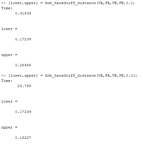
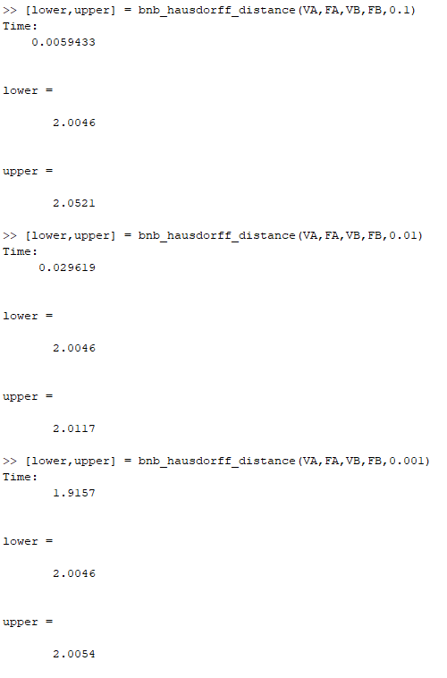
Results
Below are our results for two simple meshes, first one being a sphere mesh and the second one being the simple mesh found in the blog post linked under the “Discarding and subdividing” section.
Conclusion
The intuition behind how to determine the Hausdorff distance is relatively simple, however the implementation of computing this distance isn’t trivial. Among the 3 tasks of this Hausdorff distance algorithm (finding the lower bound, finding the upper bound, and finding a triangular subdivision routine), the latter two tasks were dependent on finding the lower bound. We at first thought that the subdivision routine would be the most complicated process, and the lower bound would be the easiest. We were very wrong: the lower bound was actually the most challenging aspect of our code. Finding vertex-vertex distances was the easiest aspect of this computation. Given that in MATLAB triangular meshes are represented as faces of vertex points, it is difficult to identify specific non-vertex points of some triangle. To account for this, we at first used computations dependent on finding a series of normals amongst points. This yielded a functional, albeit slow, algorithm. Upon comparison, the lower bounds computation was the cause of this latency and needed to be improved. At this point, it was a matter of finding a different implementation. It was fun brainstorming with each other about possible ways to do this. It was more fun to consider counterexamples to our initial ideas, and to proceed from there. At a certain point, we incorporated geometric ideas (using the centroid of triangles) and topological ideas (using the closed balls) to find a subset of relevant faces relative to some vertex of the first mesh, instead of having to consider all possible faces of the secondary mesh. Bryce’s part was having to mathematically prove his argument, for it to be correct, but only to find out later it would be not feasible to implement (oh well). Currently, we are trying to resolve bugs, but throughout the entire process we learned a lot, had fun working with each other, and gained a stronger understanding of techniques used within geometry processing.
In conclusion, it was really fascinating to see the connection between the theoretical ideas and the implementation of an algorithm, especially how a theoretically simple algorithm can be very difficult to implement. We were able to learn more about the topological and geometric ideas behind the problem as well as the coding part of the project. We look forward to finding more robust ways to code our algorithm, and learning more about the mathematics behind this seemingly simple measure of the geometric difference between two meshes.