By SGI Fellows Xinwen Ding, Josue Perez, and Elshadai Tegegn
During the second week of SGI, we worked under the guidance of Prof. Yusuf Sahillioğlu to detect planes and edges from a given point cloud. The main tool we applied to complete this task is the Random Sample Consensus (RANSAC) algorithm.
Definition
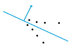
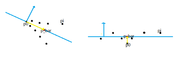
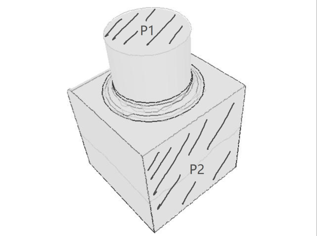
We define a plane P as the dominant plane of a 3D point cloud if the number of points defined in the 3D point cloud located on the plane P is no less than the number of points on any other plane. For example, consider the following object defined by a 3D point cloud. If we assume the number of points on a face is proportional to the area of the face, then \(P_2\) is more likely to be the dominant plane than \(P_1\) since the area of \(P_2\) is greater than that of \(P_1\). So, compared with \(P_1\), there are more points on \(P_2\), which makes \(P_2\) the potential dominant plane.
Problem Description
Given a 3D point cloud as the input model, we aim to detect all the planes in the model. To obtain a decent detection result, we divide the problem into two separate parts:
- Part 1: Find the dominant plane \(P\) from a given 3D point cloud. This subproblem can be solved by the RANSAC Algorithm.
- Part 2: Find all other planes contained in the 3D point cloud. This subproblem can be successfully addressed if we iteratively repeat the following two steps: (1). remove all the points on plane \(P\) (obtained from Part 1) from the given point cloud. (2). repeat the RANSAC algorithm with respect to the remaining points in the point cloud.
The RANSAC Algorithm
An Introduction to RANSAC
The RANSAC algorithm is a learning technique that uses random sampling of observed data to best estimate the parameters of a model.
RANSAC divides data into inliers and outliers and yields estimates computed from a minimal set of inliers with the most outstanding support. Each data is used to vote for one or more models. Thus, RANSAC uses a voting scheme.
Workflow & Pseudocode
RANSAC achieves its goal by repeating the following steps:
- Sample a small random subset of data points and treat them as inliers.
- Take the potential inliers and compute the model parameters.
- Score how many data points support the fitting. Points that fit the model well enough are known as the consensus set.
- Improve the model accordingly.
This procedure repeats a fixed number of times, each time producing a model that is either rejected because of too few points in the consensus set or refined according to the corresponding consensus set size.
The pseudocode of the algorithm is recorded as below:
function dominant_plane = ransac(PC)
    n := number of points defined in point cloud PC

    max_iter := max number of iterations

    eps := threshold value to determine data points that are
           fit well by model (a 3D plane in our case)

    min_good_fit := number of nearby data points required to
                    assert that a model (a 3D plane in our
                    case) fits well to data

    iter := current iteration

    best_err := measure of how well a plane fits a set of
                points. Initialized with a large number

    % store dominant plane information
    % planes are characterized as [a,b,c,d], where
    % ax + by + cz + d = 0
    dominant_plan = zeros(1,4);

    while iter < max_iter
        maybeInliers := 3 randomly selected values from data
        maybePlane := a 3D plane fitted to maybeInliers
        alsoInliers := []
        for every point in PC not in maybeInliers
            if point_to_model_distance < eps
                add point to alsoInliers
            end if
        end for

        if number of points in alsoInliers is > min_good_fit
            % the model (3D plane) we find is accurate enough

            % this betterModel can be found by solving a least
            % square problem.
            betterPlane := a better 3D plane fits to all
                        points in maybeInliers and alsoInliers
            err := sum of distances from the points in
                   maybeInliers and alsoInliers to betterPlane
            if err < best_err
                best_err := err
                dominant_plane := betterPlane
            end if
        end if

        iter = iter + 1;
    end while
end
Detect More Planes
As mentioned before, to detect more planes, we may simply remove the points that are on the dominant plane \(P\) of the point cloud, according to what is suggested by the RANSAC algorithm. After that, we can reapply the RANSAC algorithm to the remaining points, and we get the second dominant plane, say \(P’\) of the given point cloud. We may repeat the process iteratively and detect the planes one by one until the remaining points cannot form a valid plane in 3D space.
The following code provides a more concrete description of the iterative process.
% read data from .off file
[PC, ~] = readOFF('data/off/330.off');

% A threshold eps is set to decide if a point is on a detected
% plane. If the distance from a point to a plane is less than
% this threshold, then we consider the point is on the plane.
eps = 2e-3;

while size(PC, 1) > 3
    % in the implementation of ransac, if the algorithm cannot
    % detect a plane using the existing points, then the
    % coefficient of the plane (ax + by + cz + d = 0) is a
    % zero vector.
    curr_plane_coeff = ransac(PC);

    if norm(curr_plane_coeff) == 0
        % remaining points cannot lead to a meaningful plane.
        % exit loop and stop algorithm
        break;
    end

    % At this point, one may add some code to visualize the
    % detected plane.

    % return the indices of points that are on the dominant
    % plane detected by RANSAC algorithm
    [~, idx] = pts_close_to_plane(PC, curr_plane_coeff, eps);

    % remove the points on the dominant plane.
    V(idx,:) = [];
end
Results
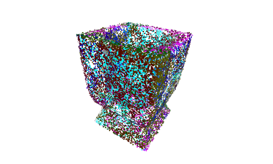
RANSAC algorithm gives good results with 3D point clouds that have planes made up of a good number of points. The full implementation is available on SGI’s Github. This method is not able to detect curves or very small planes. The data we used to generate these examples are the Mechanical objects (Category 17) from this database.
Successful Detections
| Mech. Data Model Number | Model Object | RANSAC Plane Detection Result |
| 330 | 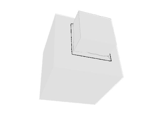 | 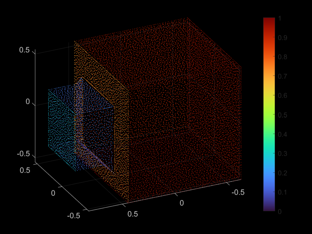 |
| 331 | 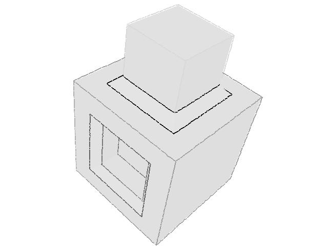 | 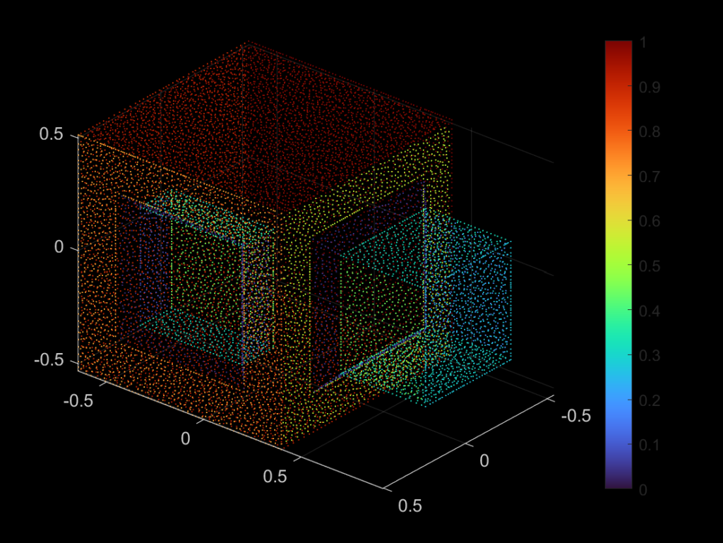 |
Unsuccessful Detections
| Mech. Data Model Number | Model Object | RANSAC Plane Detection Result |
| 332 | 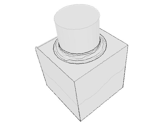 | 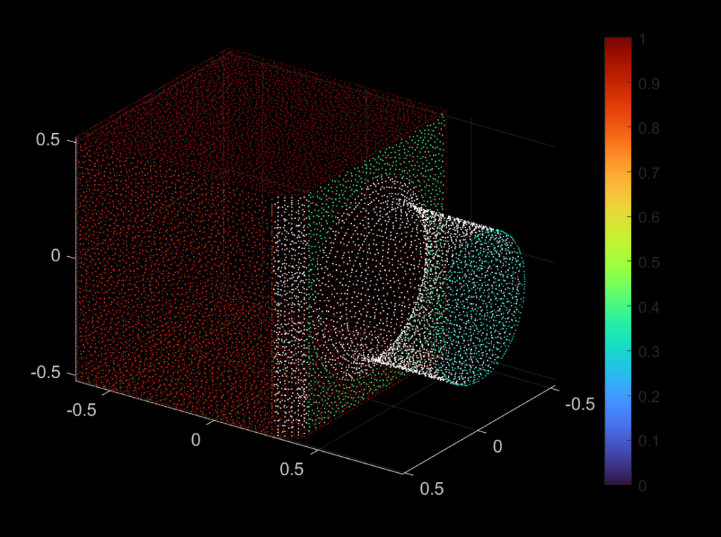 |
| 338 | 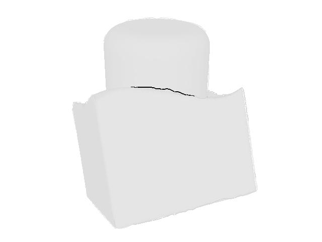 | 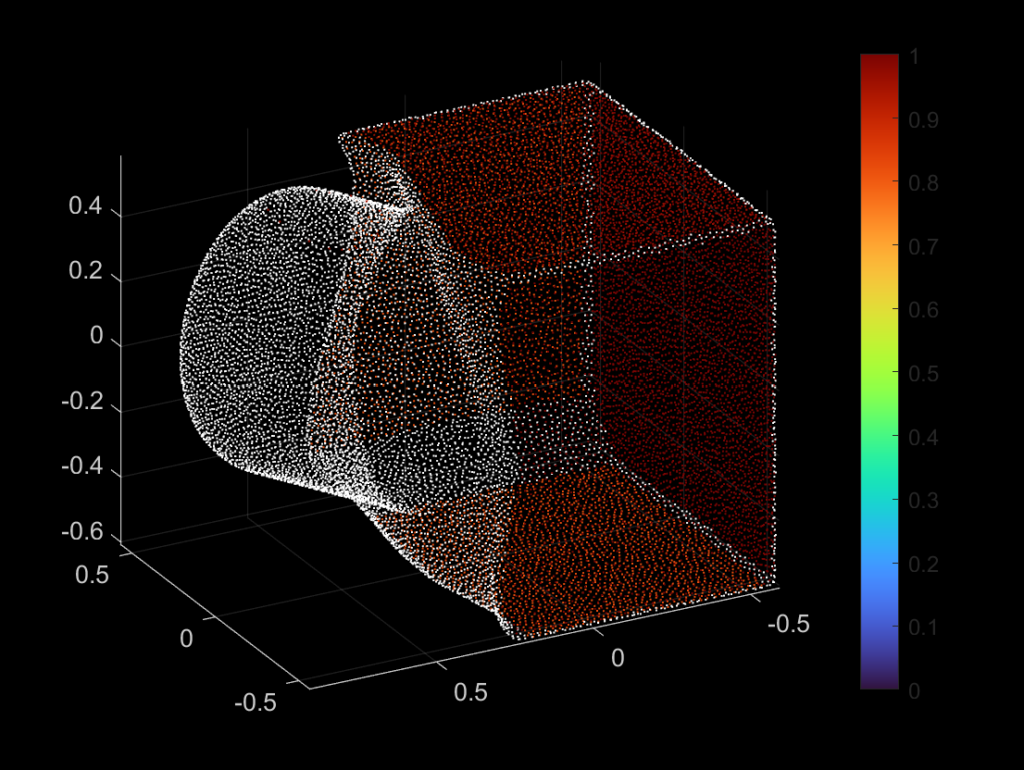 |
Limitations and Future Work
As one may observe from the successful and unsuccessful detections, the RANSAC algorithm is good at detecting planar surfaces. However, the algorithm usually fails to detect a curved surface, because we are fitting the three randomly selected points using a plane equation as our base model. If we change this model to be a curved surface, then theoretically speaking, the RANSAC algorithm should be able to detect a curved plane. We may apply a similar fix if we want to perform line detection.
Moreover, we may notice that the majority of surfaces in our test data can be represented easily by an analytical formula. However, this pre-condition is, in general, not true if we choose an arbitrary point cloud. If this is the case, the RANSAC algorithm is unlikely to output an accurate detection result, which leads to more extra work.