by Jayati Sood, Uriel Martínez, Miles Silberling-Cook and Josue Perez
Introduction
The geodesic distance between two points x and y on a mesh is the length of the shortest path from x to y, along the surface. In the first and final weeks of SGI, under the mentorship of Professor Justin Solomon and Professor Nester Guillen, we worked on finding numerical approximations of geodesic distance functions that are low in accuracy and hence faster to compute.
Given a point a set \(S\) of points on the surface \(\mathcal{M}\), we can define a function \(f_S(x):\mathcal{M}\mapsto\mathbb{R}^+\) such that
\[f_S(x) = d(x, S) = \min_{y\in S} d(x,y),\]
where \(d\) is the geodesic distance function in \(\mathcal{M}\). \(f\) satisfies the eikonal equation, i.e.,
\[||\nabla f(x)||_2=1.\]
Solving the eikonal equation with \(f_{S}(x_0)=0\) gives us the geodesic distance function from a given set of points on the mesh/manifold to all other points on the mesh. However, the eikonal equation is a non-linear PDE and hard to solve. To speed up the process, we employ Perron’s method to solve for \(f_{S}(x)\) by finding the maximum of the subsolutions of the above boundary value problem, which leads to the following convex optimization problem:
\begin{align*} \max_f & \;\; \int_{\mathcal{M}}f(x)dx \\ \text{subject to } & \;\; f(x) \leq 0\;\forall\;x\in S \\ & \;\;|\nabla f(x)| \leq 1\; \forall\;x \in \mathcal{M}\hspace{3.3cm} \end{align*}
Discretizing the problem
Our first task was to reformulate this optimization problem for triangle meshes. By restricting paths to the edges of the mesh we arrive at the following. Take our triangle mesh to be an edge-weighted, undirected graph \(G\).
If \(S\subset G\) is the set of vertices to which we are calculating a geodesic, then the distance function \(x\mapsto d(x, S)\) is the unique solution of the following second-order cone program (SOCP):
\[ \begin{align*} \max_f& \;\; \sum \limits_{i=1}^N f(x_i) \\ \text{subject to } & \;\; f(x_i) = 0\;\forall\;x_i\in S \\ & \;\;f(x_i)-f(x_j) \leq \ell_{e} \text{ anytime } e := (x_i,x_j) \in E \end{align*} \]
We can observe from the formulation of the problem that we have two types of constraints. The number of equations we have of the first kind depends directly on the cardinality of \(S\), meanwhile, the number of equations we have of the second type depend on the cardinality of the edges on the mesh. Hence an upper bound on the number of constraints of this particular problem is \(|S|+|E|=\frac{|S|(|S|+1)}{2}\). In other words, the number of constraints in our problem grows quadratically on the amount of vertices on the mesh. Furthermore, there is no good reason why \(f\) should be linear in general, which makes solving this problem even more computationally taxing.
We found that this formulation of the problem (with paths restricted to edges) resulted in poor-quality geodesics with negligible increase in speed. For the remainder of this project we used a form closer to the original, and approximated the gradient with finite differences. Our observations about the number of constraints still apply.
Approach
The approach we took on this project to solve these inconveniences proceeds twofold.
On a first instance, we represent \(f\) in terms of a convenient linear basis, just only for building an approximate notion of distance which takes into account only the elements on the basis that influence the most the values of \(f\), in other words, we build a low resolution geodesic. For selecting this linear base we start calculating the laplacian of the mesh. Then, we select a fixed number of eigenvectors of the matrix, giving preference to those with a lower eigenvalue.
On a second instance, we require the solution of our problem to be of low resolution. We do this by imposing new linear constraints. This could be thought to be contradictory with the goal of the project, however, with the proper use of some standard tools of convex optimization, for example the active set method, in theory we could actually reduce the number of constraints in the original problem. A consequence that we observed by using this approach on reasonably behaved meshes is that the number of active constraints on the problem depends on the size of sampled basis, yielding a method that is almost independent of the cardinallity of \(S\).
Throughout the project, we used cvx in MATLAB to solve our convex program for different sets \(S\) of vertices on the mesh, concluding with \(S\) being the set of all vertices on the mesh, which gave us the distance function for all pairs of vertices. Over the course of the project, we employed various techniques to increase the efficiency of our solver, and were successful in obtaining an all-pairs geodesic distance function on the Spot mesh.
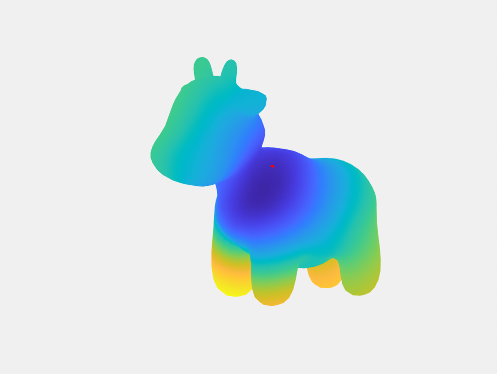
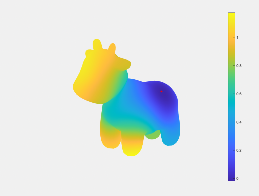
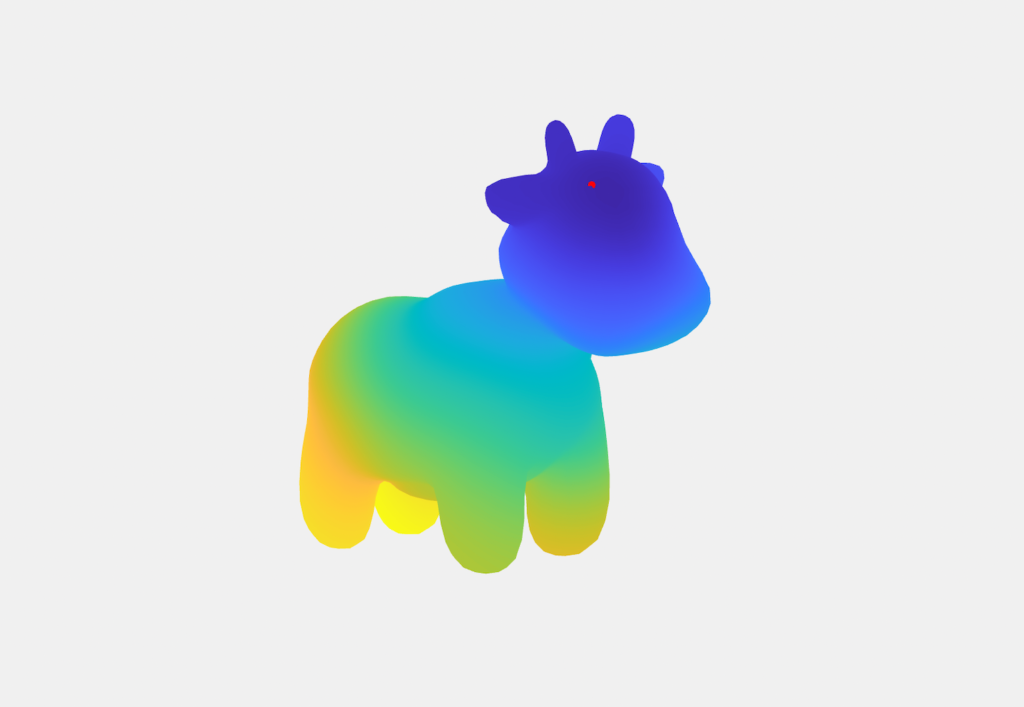
Geodesic distance function heat map
This heat map is a plot of the approximate all-pairs geodesic function for a vertex randomly sampled from Spot. The colour values represent the estimated geodesic distance from the sample vertex (red).
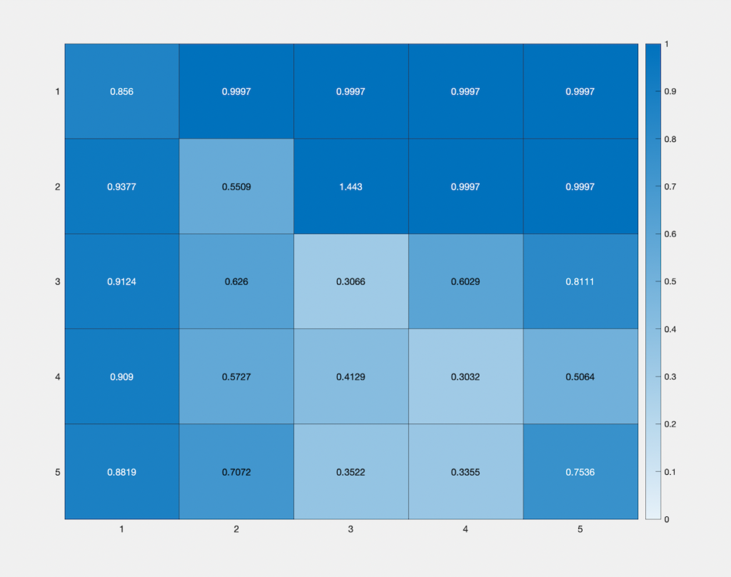
Error map
This heat map represents the change in accuracy of our approximate all-pairs geodesic distance function, with change in the number of basis vectors (vertical), and number of faces sampled (horizontal) from the Spot mesh. The colour values represent the mean relative error between the approximated function and the ground truth geodesic function, with the lightest and darkest blues being assigned to the error values “0” and “1.5”, normalized according to the observed distribution of the error values obtained. Starting with 5 faces and 5 basis vectors, and taking intervals of 5 for both, we observe that the highest accuracy is obtained along the diagonal, i.e, when the number of faces sampled equals the number of basis vectors.