In industry CAD (Computer-Aided Design) representation for 3D models is very used, and it is estimated that about 80% of overall analysis time is devoted to mesh generation in the automotive, aerospace and shipbuilding industries. But, the geometric approximation can lead to accuracy problems and the construction of the finite element geometry is costly, time-consuming and creates inaccuracies.
Isogeometric Analysis (IGA) is a technique that integrates FEA (Finite Element Analysis) into CAD (Computer-Aided Design) models, enabling the model to be designed and tested using the same domain representation. IGA is based on NURBS (Non-Uniformal RAtional B-Splines) a standard technology employed in CAD systems. One of the benefits of using IGA is that there is no approximation error, as the model representation is exact, unlike conventional FEA approaches, which need to discretize the model to perform the simulations.
For our week 4 project we followed the pipeline described in Yuxuan Yu’s paper [1], to convert conventional triangle meshes into a spline based geometry, which is ready for IGA, and we ran some simulations to test it.
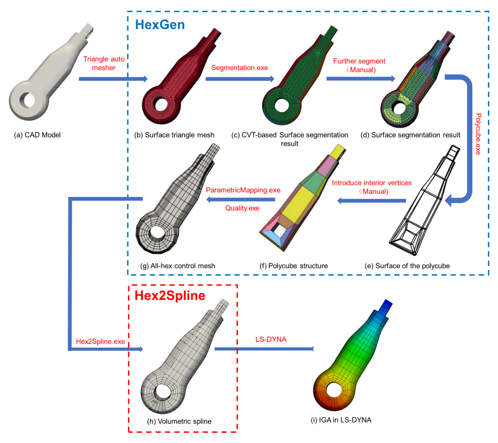
The general pipeline consists of two parts: the HexGen, which transforms a CAD Model into a All-Hex Mesh, and the Hex2Spline, which transforms the All-Hex Mesh into a Volumetric Spline, ready for IGA. The code can be found here GitHub – SGI-2022/HexDom-IGApipeline.
HexGen and Hex2Spline pipeline
Following the pipeline
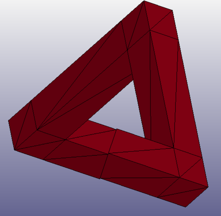
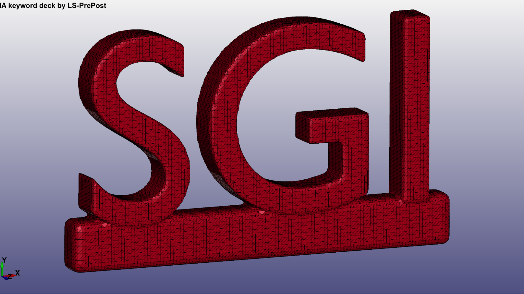
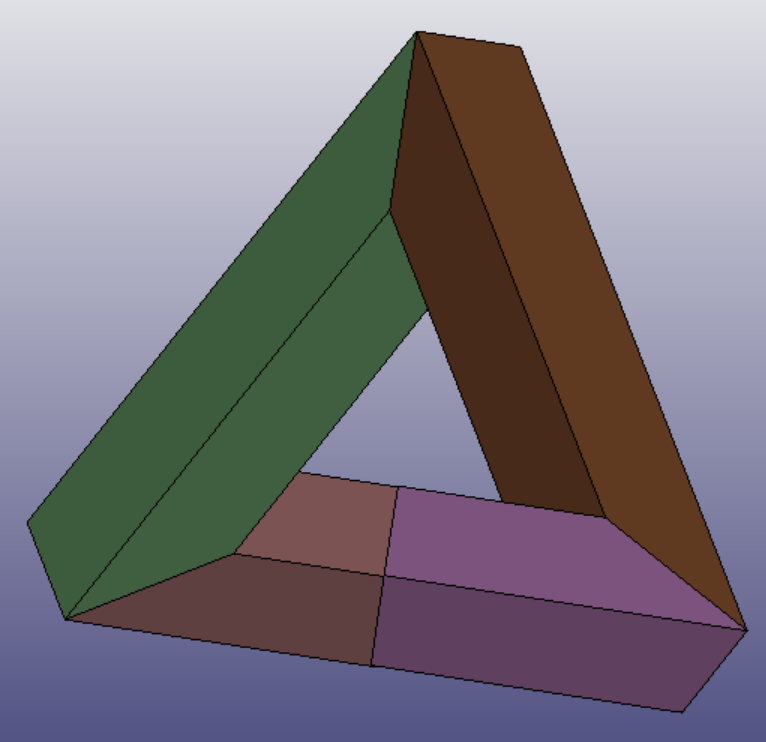
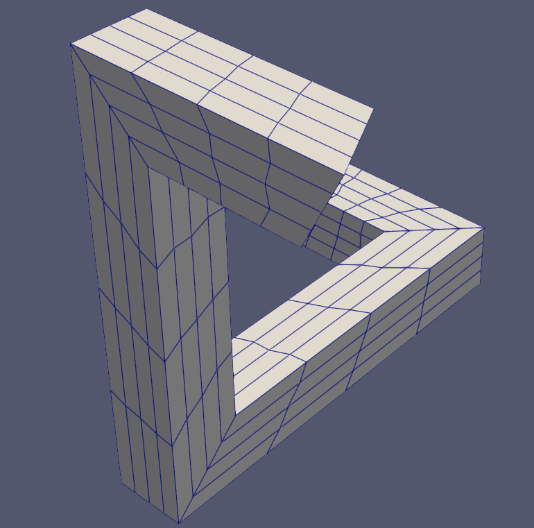
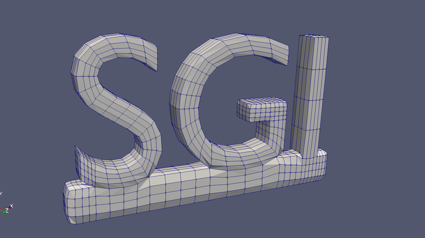
For testing the pipeline, we reproduced the steps with our own models. LS-prepost was used to visualize and edit the 3D models. We started with two surface triangle mesh:
Penrose triangle meshSGI triangle mesh
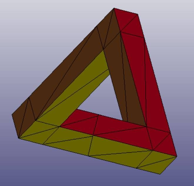
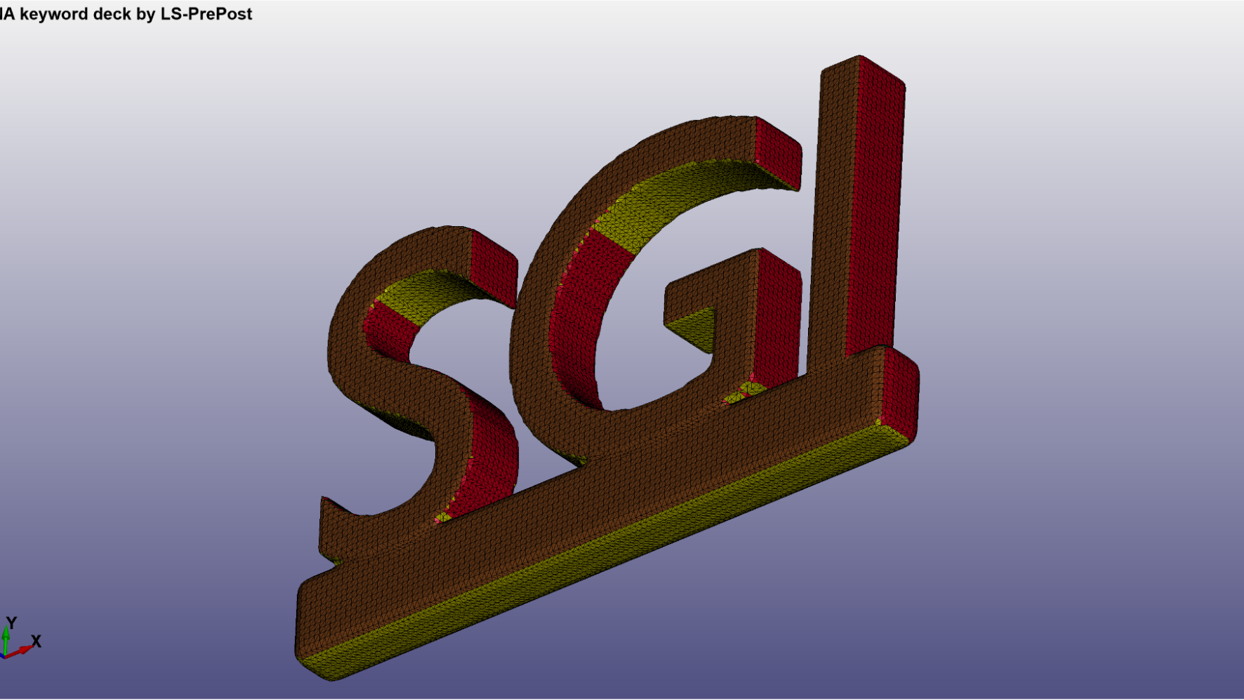
The first step of the pipeline is using a surface segmentation algorithm based on CVT (Centroidal Voronoi Tessellation), using the Segmentation.exe script. It was used to segment the triangle mesh into 6 regions, one for each of the three principal normal vectors and their opposite normals (±𝑋, ±𝑌, ±𝑍).
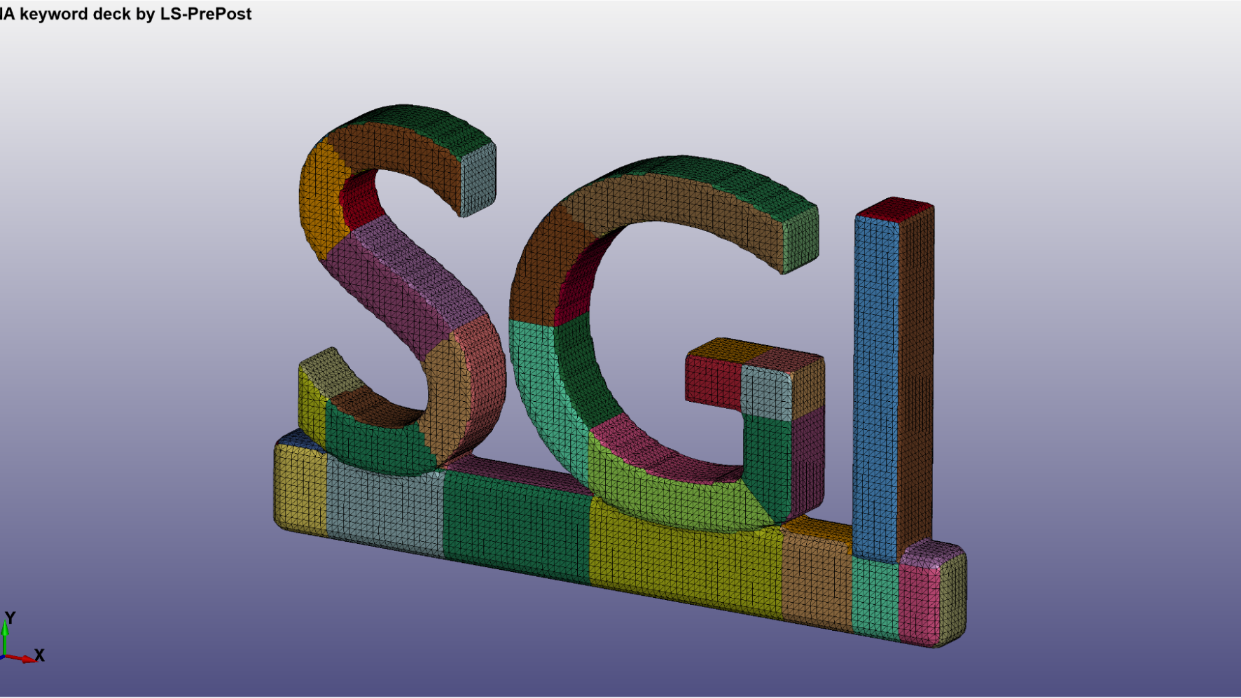
The initial segmentation only generates 6 clusters, and for more complex shapes we need a better segmentation to later build a polycube structure. Therefore, a more detailed segmentation is done, trying to better divide the mesh into regions that can be represented by polycubes. This step is done manually.
Penrose segmentationSGI segmentation
Now it is clearly visible which are the faces for the polycube structure. We can now apply a linearization operation on the segmentation, using the Polycube.exe script.
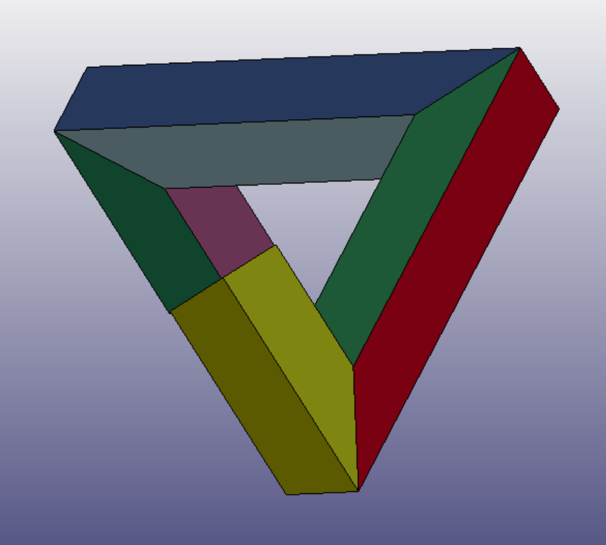
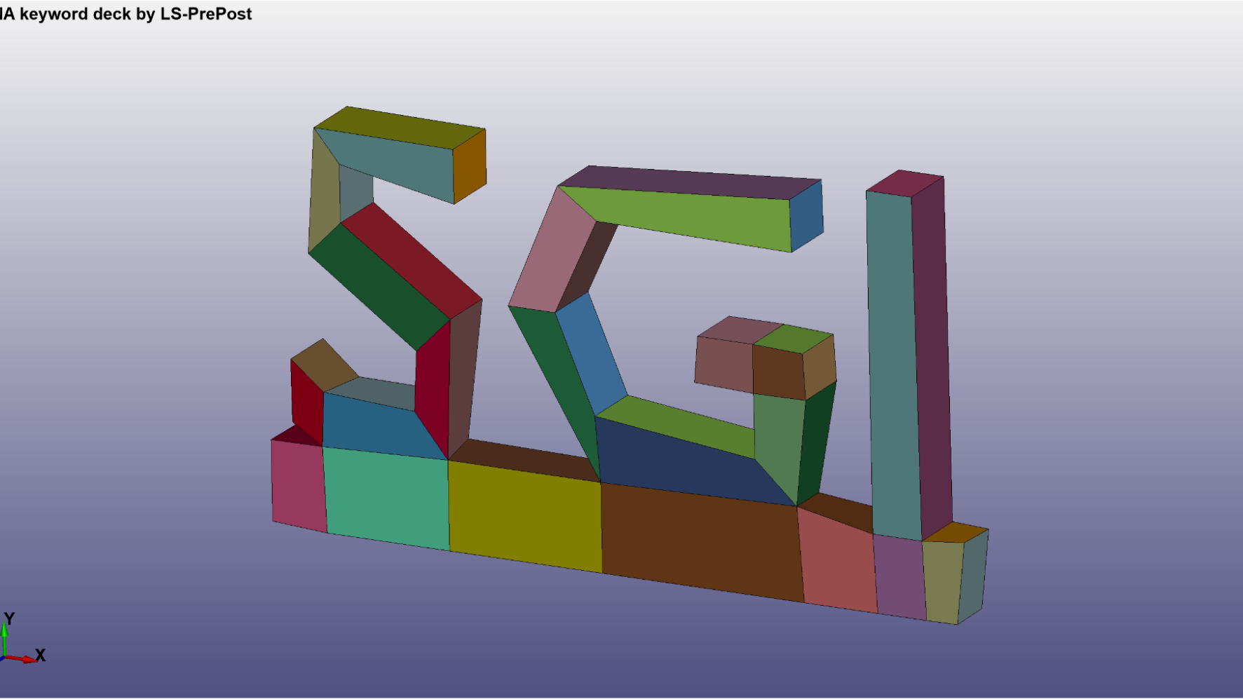
After that, we join the faces to create the cubes and finally have our polycube structure. This step is also done manually. The image in the right represents the cubes decreased in volume, for better visualization.
Penrose polycube structureSGI polycube structure
Then we want to build a parametric mapping between polycube and CAD model, which takes as input the triangle mesh and the polycube structure, to create an all-hex mesh. For that, we use the ParametricMapping.exe script.
Penrose all-hex meshSGI all-hex mesh
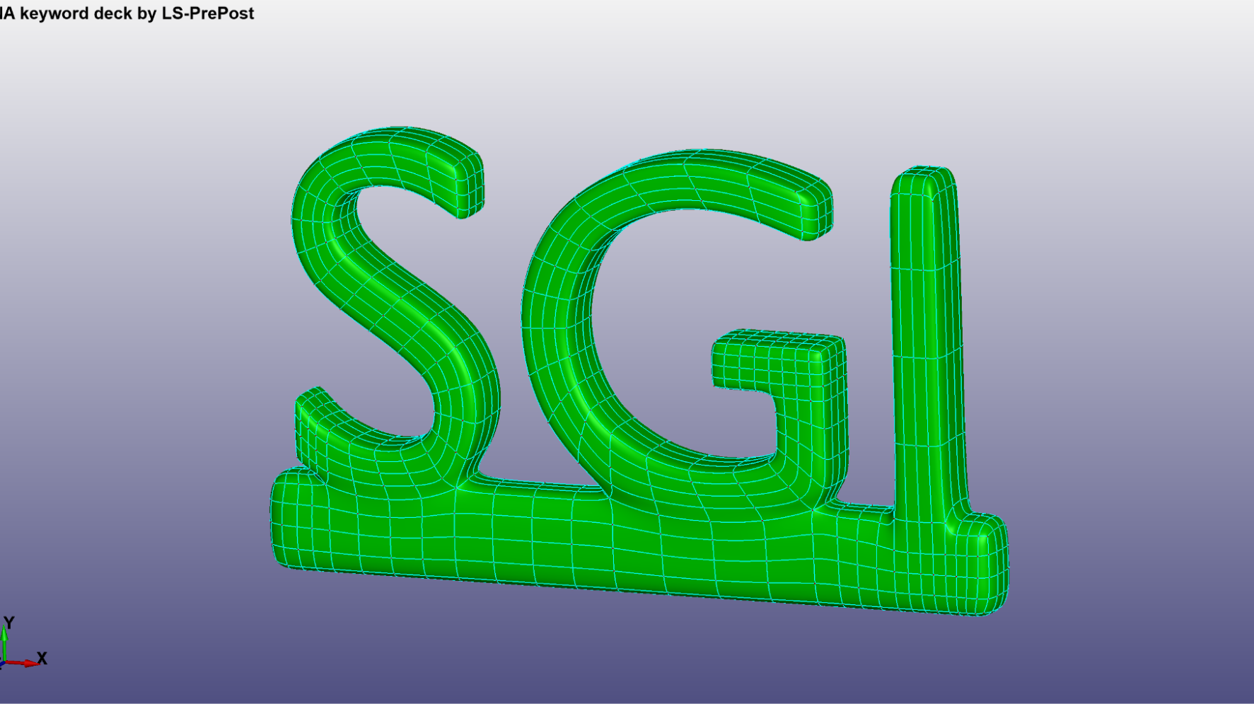
And in the last step, we use the Hex2Spline.exe script to generate the splines.
Penrose splineSGI spline
For testing the Splines, we performed a Modal Analysis (simple eigenvalue problem) in each of them, using the LS-DYNA simulator. An example for a specific displacement can be seen below:
Penrose modal analysis
SGI modal analysis
Improvements for the pipeline
The pipeline used still have two manual steps: the segmentation of the mesh, and building the polycube structure given the linear surface segmentation. During the week, we thought and discussed some possible approaches to automate the second step. Given the external faces of the polycube structure, we need to recover the volumetric information. We came up with a simple approach using graphs, representing the polycubes as vertices, the internal faces as edges, and using the external faces to build the connectivity between the polycubes.
Although, this approach doesn’t solve all the cases, for example, when a polycube consists mostly of internal faces, and are not uniquely determined. And even if we automated this step, the manual segmentation process still is a huge bottleneck in the pipeline. One solution to the problem would be generating the polycube structure directly from the mesh, without the need of a segmentation, but it’s a hard problem to automatically build a structure that doesn’t have a big amount of polycubes and still represents well the geometry and topology of the mesh.
By Tiago Fernandes, Anna Krokhine, Daniel Scrivener, and Qi Zhang
During the first week of SGI, our group worked with Professor Misha Kazhdan on a virtually omnipresent topic in the field of geometry processing: algorithmically assigning normal orientations to point clouds.
Introduction
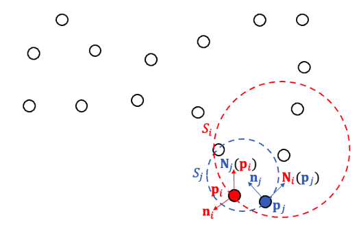
While point clouds are the typical output of 3D scanning equipment, triangle meshes with connectivity information are often required to perform geometry processing techniques. In order to convert a point cloud to a triangle mesh, we first need to orient the point cloud — that is, assign normals \(\{n_1, … n_n\}\) and signs \(\{\alpha_1, … \alpha_n\}\) to the initially unoriented points \(\{p_1, … p_n\}\).
To find \(n_i\), we can locally fit a surface to each point \(p_i\) using its neighborhood \(N(i)\) and use its uniquely determined normal. More difficult, however, is the process of assigning consistent signs to the normals. In order to evaluate the consistency of the signs, we have the following energy function, which we minimize over alpha:
\(E(\alpha)=\alpha^T\cdot E\cdot \alpha\)
Where \(\alpha \in \{-1, +1\}^n\) is the vector of signs and \(\tilde{E}_{ij} = \begin{cases} \frac{\langle N_i(p_i), N_i(p_j)\rangle \cdot \langle N_j(p_i), N_j(p_j) \rangle}{2} & i \sim j \\ 0 & \text{otherwise}\end{cases}\).
Two neighboring points, labelled pi and pj, have their normal orientations determined by the mapping of each normal onto the other point’s best-fit surface.
As shown in the diagram, \(N_i(p_j)\) is the normal assigned to \(p_j\) by the local surface fitted at \(p_i\). Greater values of \(E_{ij}\) indicate more consistent normal orientations, and thus we encourage neighboring points to have similar orientations.
Our goal is to obtain a set of signs minimizing this energy function, which is difficult to calculate on the full point set at once. To simplify the process, we looked at algorithms built on a hierarchical approach: we solve the problem first on small clusters of points, recursively building larger solutions until we’ve arrived at the initial problem.
Within this general algorithmic structure, we explored different possibilities as to the surfaces used to represent each cluster of points locally. Prof. Kazhdan had previously tried two approaches, one linear and the other quadratic. The linear approach assigns best-fit planes to the neighborhood around each point, whereas the quadratic approach uses general quadratic functions of best fit.
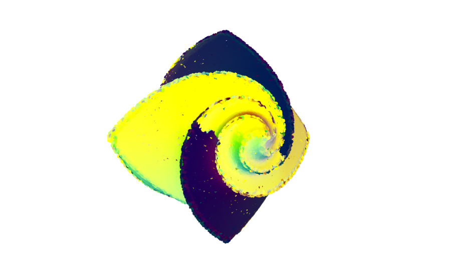
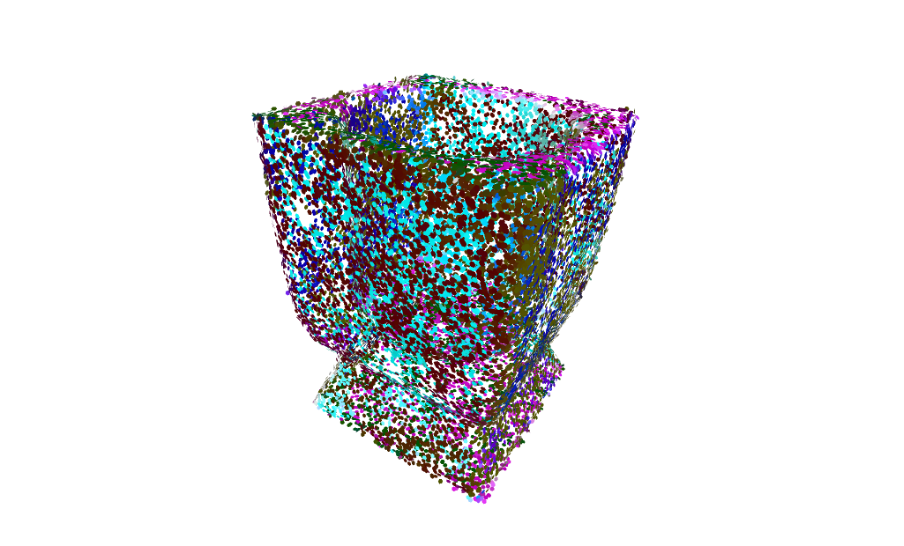
While these techniques provided a good foundation, we identified several failure cases upon experimenting with various point clouds. The linear approach works well on simple faces, but struggles to maintain consistent orientation around sharp features like edges. This is best demonstrated with the flower pointset, where the orientations of the normals are inverted in some clusters. The quadratic approach does better with fitting to distinctive features but overfits to what should be more simple surfaces, producing some undesirable outcomes such as the flower and vase seen below.
flower.xyz generated with linear fitting
Vase generated with quadratic fitting
Defining New Fits: First Attempt
Given that the linear and quadratic fits presented their own unique shortcomings, it became clear that we needed to experiment with different surface representations in order to find suitable fits for all clusters. Thanks to the abstract nature of our framework, there were few limitations on how the implicit surface needed to be defined; the energy function requires only a method for querying the gradient as well as a means of flipping the gradient’s sign, which leaves many options for implementation.
Our first geometric candidate was the sphere, a shape that approximates corners well due to the fact that it has curvature in all three directions. Additionally, fitting a set of points to a sphere is fairly straightforward: we used the least-squares approach described here, which, in implementation terms, is no more difficult than setting up a linear system and solving it. Unfortunately, the simplest solutions are not always the best solutions…
flower.xyz generated with spherical fitting
The spherical fitting wasn’t able to deal with sharp edges as expected, incorrectly matching the normal orientations when merging clusters close to those edges. It also generated some noise across the surface. But the process of designing the spherical fit gave us a solid idea on how to model other surfaces (and also helped to demystify some esoteric C++ conventions).
Parabolic Fit
We’ve established that since the surface may curve, a linear fit can be non-faithful to the features of the original pointset. Conversely, the generic quadratic fit has the potential to produce undesirable surface representations such as hyperbolas or ellipsoids. To this end, we introduced a parabolic fit, which improves upon the linear fit via the addition of a parameter.
By constructing a local coordinate frame where the normal from the linear fit serves as our z-axis, we were able to fit \(z=a(x^2 + y^2)\) with energy \(E_{loss} = \sum\limits_{i} (z_i – a(x_i^2+y_i^2))^2\). From this we obtained \(a = \frac{\sum_i z_i (x_i^2+y_i^2 ) }{\sum_i(x_i^2+y_i^2 )^2}\) yielding an \(a\) that minimizes this energy. By observing that \(z_i=\langle \vec{p_0 p_i} ,n \rangle, x_i^2+y_i^2=||\vec {p_0 p_i} \times n||^2\) , we derived a formula that is easier to represent programmatically: \(a = \frac{\sum_i \langle \vec{p_0 p_i} ,n \rangle ||\vec {p_0 p_i} \times n||^2 }{\sum_i||\vec {p_0 p_i} \times n||^4}\).
We calculated the gradient in a similar manner. Since locally \(\nabla ( z – a(x^2+y^2)) = (-2ax,-2ay,1) = -2a(x,y,0) + (0,0,1)\), then \(\nabla ( z – a(x^2+y^2)) = -2a\cdot \mbox{Proj}(\vec{p_0 p_i}) + \vec{n}\), where \(\mbox{Proj}( )\) projects vectors into the plane obtained in the original fit, which is written in a more code-friendly manner as \(\mbox{Proj}(\vec{x}) = \vec{x} – \langle \vec{x}, \vec{n} \rangle \vec{n}\). Finally, the gradient could be expressed as \(\nabla ( z – a(x^2+y^2)) = -2a(\vec{x} – \langle \vec{x}, \vec{n} \rangle \vec{n}) + \vec{n}\).
Our implementation of the parabolic fit generally works better than the linear fit, correcting for some key errors. It works particularly well on smooth, curved point clouds.
As for the flower dataset, however, the performance was still sub-par. When we examined some of the parabolic fits using a tool to visualize the isosurface, we found the following problem with some of the normals:
The normal of the best-fit plane doesn’t align with the best-fit parabola.
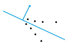
In this example, \(\vec{p_0 \bar p}\) would serve as a better normal vector than \(\vec{n}\), so we decided to implement a “choice” between the two. To avoid swapping the normal on flat point clouds (where the original normal serves its purpose quite well) we determined a threshold to handle this. Intuitively, a point cloud encoding an edge will yield a larger \(||\vec{p_0 \bar p}||\):
Two cases: one in which the cluster encodes an edge (left), and one in which the cluster encodes a plane (right)
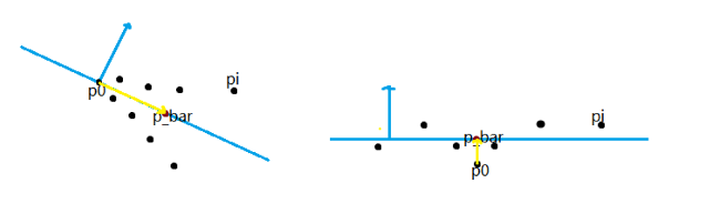
To obtain a good threshold value, we used the local radius \(d_{max} = \max _{i} ||\vec{p_0 p_i}||\) and then picked a $ c$ that seems to work with our dataset (related to the size of each neighborhood), such that when \(||\vec{p_0 \bar p}|| < d_{max}/c\), we can assume the cluster is flat, whereas when \(||\vec{p_0 \bar p}||\ge d_{max}/c\) we expect it to be sharp.
Another comparison of the two cluster cases (angular versus flat local geometry). Note the relative sizes of p_bar and dmax.
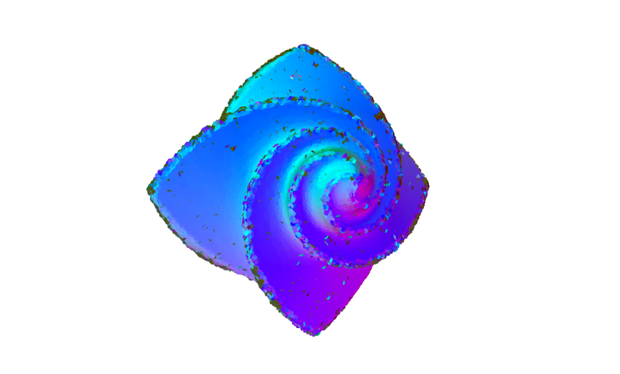
In practice, this idea works well on flower.xyz when \(c \ge 12\) — the parameter is rather sensitive and can yield poor results on some point clouds if not tuned properly.
flower.xyz with parabolic fitting
Hybrid Methods: The Associative Fit
The parabolic fit provided a lot of hope as to how we could definitively address large variations in curvature. Recalling that the quadratic fit worked well for some types of clusters and that the linear fit worked well for others, the advantages of somehow being able to merge the two methods by leveraging both of their strengths had become apparent. This observation is what ultimately gave rise to the “associative” fit, which
constructs two different fits for each cluster, and
chooses the best fit by comparing the performance of the first fit to a user-specified threshold value.
The first fit’s performance is assessed according to a standard statistical measurement known as R-squared, which tells us, as a percentage, how much of the point cluster’s variation is explained by the chosen fit (or simply put, the correlation between the fit and the pointset). This was straightforward enough to implement with respect to our linear fit, which always serves as the first fit that AssociativeFit attempts to query. We can completely disable the linear fit when its R-squared value does not meet the threshold for inclusion, allowing us to switch to a better fit (quadratic, parabolic) for clusters where the observed variance is too great for a planar representation. As it turns out, clusters with high variance are likely to encode geometries with high curvature, which makes the use of a higher-degree fit appropriate.
Many of our best results were obtained using the associative fit, and we were pleased to see clear improvements over the original single-fit approaches. The inclusion of a threshold parameter does necessitate a lot of hands-on trial and error by the user — we’d eventually like to see this value determined automatically per-pointset, but the optimization problem involved in doing so is particularly challenging given that each point cloud has its own issues related to non-uniform sampling and density.
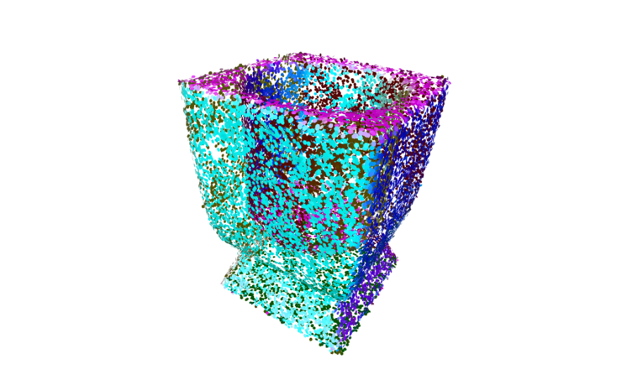
flower.xyz generated with associative (linear, quadratic) fitting
flower.xyz generated with associative (linear, quadratic) fitting
Quantitative Performance, Distance Weighting, and Other Touch-Ups
Aside from defining new implicit surfaces, we made a lot of other miscellaneous changes to the existing code base in order to improve our means of assessing each fit’s performance. We also wanted to provide the user with as much flexibility as possible when it came to manual refinement of the results.
At the beginning, when it came time to analyze our results, we relied heavily upon the disk-based visualization tool used to generate the images in this blog post. We also explored geometry processing techniques (mainly Poisson reconstruction) that make extensive use of the generated normals, assessing their performance as a proxy for the success of our method. These tools, however, provide only a qualitative means of assessment, essentially boiling down to whether a result “looks good.”
Fortunately, many of the point clouds in our dataset came with pre-assigned “true” normals that were then discarded by our method as it attempted to reconstruct them. We could easily use these normals as a point of comparison, allowing us to generate two metrics: similarity of normal lines (absolute value of the dot product, orientation-agnostic) and similarity of orientations (sign of the dot product). These statistics not only helped us with our debugging, but serve as natural candidates for any future optimization process that compares multiple passes of the algorithm.
The last main improvement to cover is the introduction of “weights” in the construction of each fit, or attenuating values that attempt to diminish the contribution of points farthest away from the mean. Despite having been implemented before we even touched the codebase, the weights were not used until we enabled them (previously, each fit received a weighting function that always returned a constant value rather than one of these distance-based weights). Improvements were modest in some cases and quite noticeable in others, as indicated by our results.
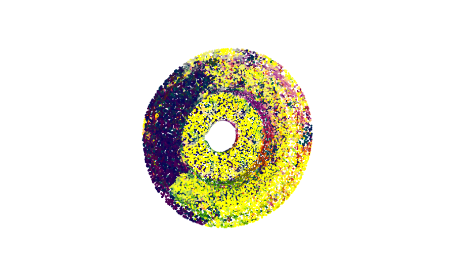
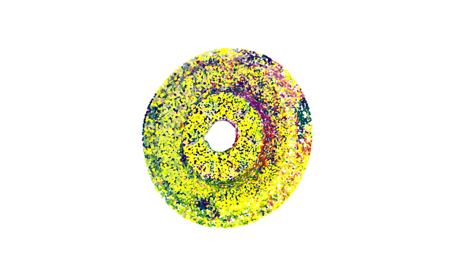
Pulley generated without distance weighting
Pulley generated with distance weighting
Conclusion
The problem of orienting point clouds is NP-hard in its simplest formulation, and a good approach for this task needs to take advantage of the geometric properties and structure of point clouds. By implementing more complex surface representations, we were able to significantly improve the results obtained across the 17 point clouds used for testing. The associative & parabolic fits in particular produced promising results: both were able to preserve the orientations of clusters across sharp edges and smooth surfaces alike.
Several obstacles remain with regard to our approach. The algorithm may perform poorly on especially dense point clouds or point clouds with non-manifold geometry. Additionally, our new surface representations are sensitive to manually-specified parameters, preventing this method from working automatically. Fortunately, the latter issue presents an opportunity for future work with optimization.
It was exciting to start off SGI working on a project with so many different applications in the field of geometry processing and beyond. The merit of this approach lies primarily with the fact that it provides an out-of-the box solution: once you compile the code, you can start experimenting with it right away (there are no neural networks to train, for example). We’re hopeful that this work will only continue to see improvements as adjustments are made to the various surface implementations (and there may be a part II on that front — stay tuned!)
Many of the SGI fellows experienced an error using the png2poly function from the gptoolbox: when applied to the example picture, the function throws an indexing error and in some cases makes Matlab crash. So, I decided to investigate the code.
The function png2poly transforms a png image into closed polylines (polygons) and applies a Laplacian smoothing operation. I found out that this operation was returning degenerated polygons, which later in the code was crashing Matlab.
But first, how does Laplacian smoothing work?
I had never seen how a smoothing operation works, and I was surprised with how simple the idea of Laplacian smoothing is. It’s an iterative operation, and at each iteration the positions of the vertices are updated using local information, the position of neighbor vertices.
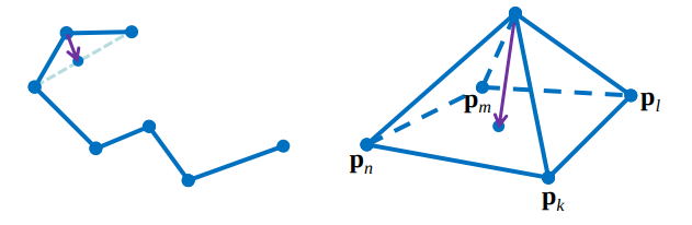
New position of vertices after one iteration (credit: Stanford CS 468).
In polylines, every vertex has 2 neighbors, apart from boundary vertices, to which the operation is not applied. For closed polylines, Laplacian smoothing converges to a single point after many iterations.
The Laplacian matrix \(L\) can be used to apply the smoothing for the whole polyline at once, and a Lambda parameter (0 ≤ λ ≤ 1) can be introduced to control how much the vertices are going to move in one iteration:
\[p \gets p + \lambda L p\]
The best thing about Laplacian smoothing is that the same idea pleasantly applies for meshes in 3D! The difference is that in meshes every vertex has a variable number of neighbors, but the same formula using the Laplacian matrix can be used to implement it.
For more details on smoothing, check out this slide from Stanford, from which the images in this post were taken. It also talks about ways to improve this technique using an average of the neighbors weighted by curvature.
What about the bug?
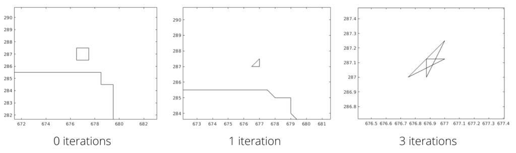
The bug was the following: For some reason, the function that converts the png into polygons was generating duplicate vertices. Later in the code, a triangulate function is used on these polygons, and the duplicate vertices by themselves make the function crash. But even worse, when smoothing is applied to a polygon with duplicate vertices, strange things happen. Here’s an example of a square with 5 vertices (1 duplicated); after 3 iterations it becomes a non-simple polygon:
You can try to simulate the algorithm to see that it happens.
Also, the lambda parameter used was 1.0, which was too high, making small polygons collapse or generating new duplicate points, so I proposed 0.5 as the new parameter. For closed curves, Laplacian smoothing will converge to a single point, making the polygon really small after many iterations, which is also a problem for the triangulation function. In most settings, these converged polygons can be erased.
Some other problems were also found, but less relevant to be discussed here. A pull request was merged into the gptoolbox repository removing duplicate points and fixing the other bugs, and now the example used in the tutorial week should work just fine. The changes I made don’t guarantee that the smoothing operation is not generating self-intersection anymore, but for most cases it does.
Fun fact: There’s a technique for finding if a polygon has self-intersection called sweep line, which works in \(O(n\log n)\)—more efficient than checking every pair of edges!
The things I learned
Laplacian smoothing is awesome.
It’s really hard to build software for geometry processing that works properly for all kinds of input. You need to have complete control over degenerate cases, corner cases, precision errors, … the list goes on. It gets even harder when you want to implement something that depends on other implementations, that may by themselves break with certain inputs. Now I recognize even more the effort of professor Alec Jacobson and collaborators for creating gptoolbox and making it accessible.
Big thanks to Lucas Valença, for encouraging me to try and solve the bug, and to Dimitry Kachkovski, for testing my code.