Vivien van Veldhuizen

By Tiago De Souza Fernandes, Bryan Dumond, Daniel Scrivener and Vivien van Veldhuizen

If you have been keeping up with some of the recent developments in artificial intelligence, you might have seen AI models that can generate images from a text-based description, such as CLIP or DALL·E. These models are able to generate completely new images from just a single text-prompt (see for example this twitter account). Models such as CLIP and DALL·E operate by embedding text and images in the same vector space, which makes it possible to frame the image synthesis as an optimization problem, ie: find an image that, when processed by a neural network, yields an embedding similar to a corresponding text embedding. A problem with this setup, however, is that it is severely underconstrained: there are many such images and some of them are not very interesting from the perspective of a human. To circumvent this issue, previous research has focused on incorporating priors into this optimization.

Over the last few weeks, our team, under the supervision of Matheus Gadelha from Adobe Research, looked into a specific instance of such constraints: namely, what would happen if the images could only be formed through a simple assembly of geometric primitives (spheres, cuboids, planes, etc)?

An Overview of the Optimization Problem

The ability to unite text and images in the same vector space through neural networks like CLIP lends itself to an intuitive formulation of the problem we’d like to solve: What image comprising a set of geometric primitives is most similar to a given text prompt?

We’ll represent CLIP’s mapping between images/text and vectors as a function, $\phi$. Since CLIP represents text and images alike as n-dimensional vectors, we can measure their similarity in terms of the angle between the two vectors. Assuming that the vectors it generates are normalized, the cosine of the angle between them is simply the dot product $\langle \phi(Image), \phi(Text) \rangle$. Minimizing this quantity with respect to the image generated from our geometric primitive of choice should yield a locally optimal solution: something that more closely approximates the desired text prompt than its neighbors.

Two sample images — a golden retriever and a 2006 Toyota Camry — alongside their respective descriptions according to CLIP. The cosine similarity of the first image relative to the prompt “a golden retriever” is 0.2690, compared to 0.1586 for the second image.

In order to get a sense of where the solution might exist relative to our starting point, we’d like all operations involved in the process of computing this similarity score to be differentiable. That way, we’ll be able to follow the gradient of the function and use it to update our image at each step.
To achieve our goals within a limited two-week timeframe, we desire rasterizers built on simple but powerful frameworks that would allow for as rapid iteration as possible. As such, PyTorch-based differentiable renderers like diffvg (2D) and Nvdiffrast (3D) provide the machinery to relate image embeddings with the parameters used to draw our primitives to the screen: we’ll be making extensive use of both throughout this project.

2D Shape Optimization

We started by looking at the 2D case, taking this paper as our basis. In this paper, the authors propose CLIPDraw: an algorithm that creates drawings from textual input. The authors use a pre-trained CLIP language-image encoder as a metric for maximizing the similarity between the given description and a generated drawing. This idea is similar to what our project hopes to accomplish, with the main difference being that CLIPDraw operates over vector strokes. We tried a couple of methods to make the algorithm more geometrically aware, the first of which is some data augmentations.

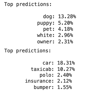
By default, the optimizer has too much creative leeway to interpret which images match our text prompt, leading to some borderline incomprehensible results. Here’s an example of a result that CLIP identifies as a “golden retriever” when left to its own devices:

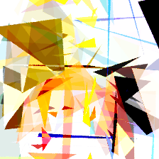
*Prompt = “a golden retriever” after 8400 iterations*

Here, the optimizer gets the general color palette right while missing out completely on the geometric features of the image. Fortunately, we can force the optimizer to approach the problem in a more comprehensive manner by “augmenting” (transforming) the output at each step. In our case, we applied four random perspective & crop transformations (as do the authors of CLIPDraw) and a grayscale transformation at each step. This forces the optimizer to imitate human perception in the sense that it must identify the same object when viewed under different ambient conditions.

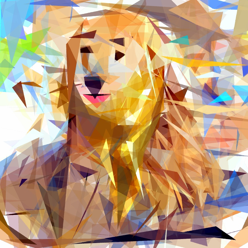
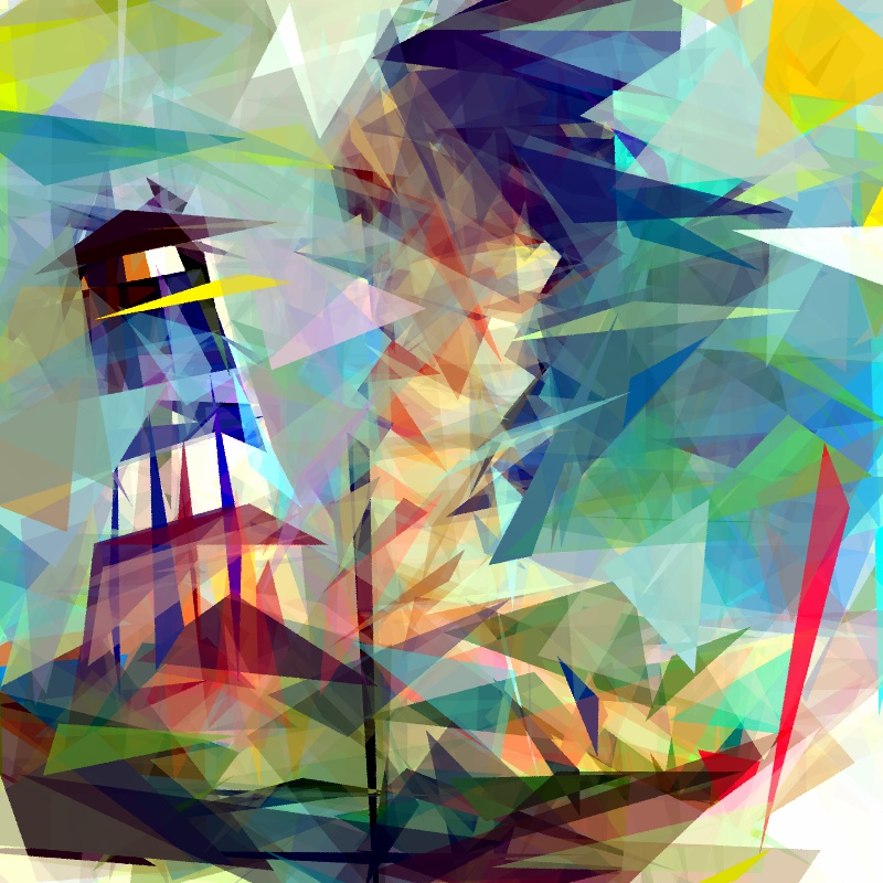
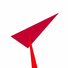
Fortunately, the introduction of data augmentations produced near-instant improvements in our results! Here is a taste of what the neural network can generate using triangles:

Generating Meshes

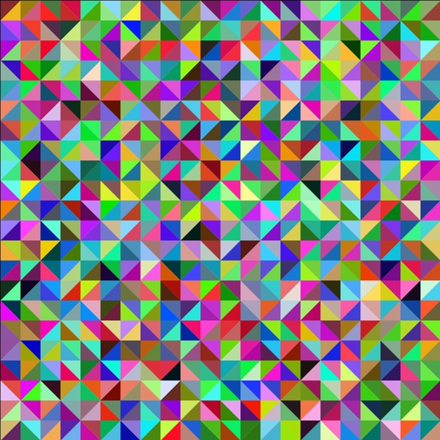
In addition to manipulating individual shapes, we also tried to generate 2D triangular meshes using CLIP and diffvg. Since diffvg doesn’t provide automatic support for meshes, we circumvented this problem using our own implementation where individual triangles are connected to form a mesh. We started our algorithm with a simple uniform randomly-colored triangulation:

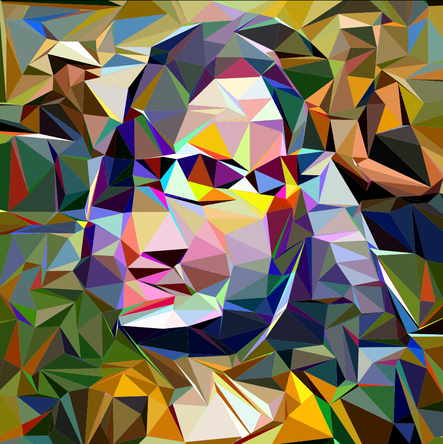
Simply following each step in the gradient direction could change their positions individually, destroying the mesh structure. So, at each iteration, we merge together vertices that would have been pushed away from each other. We also prevent triangles from “flipping”, or changing orientation in such a way that would produce an intersection with another existing triangle. Two of the results can be seen below:

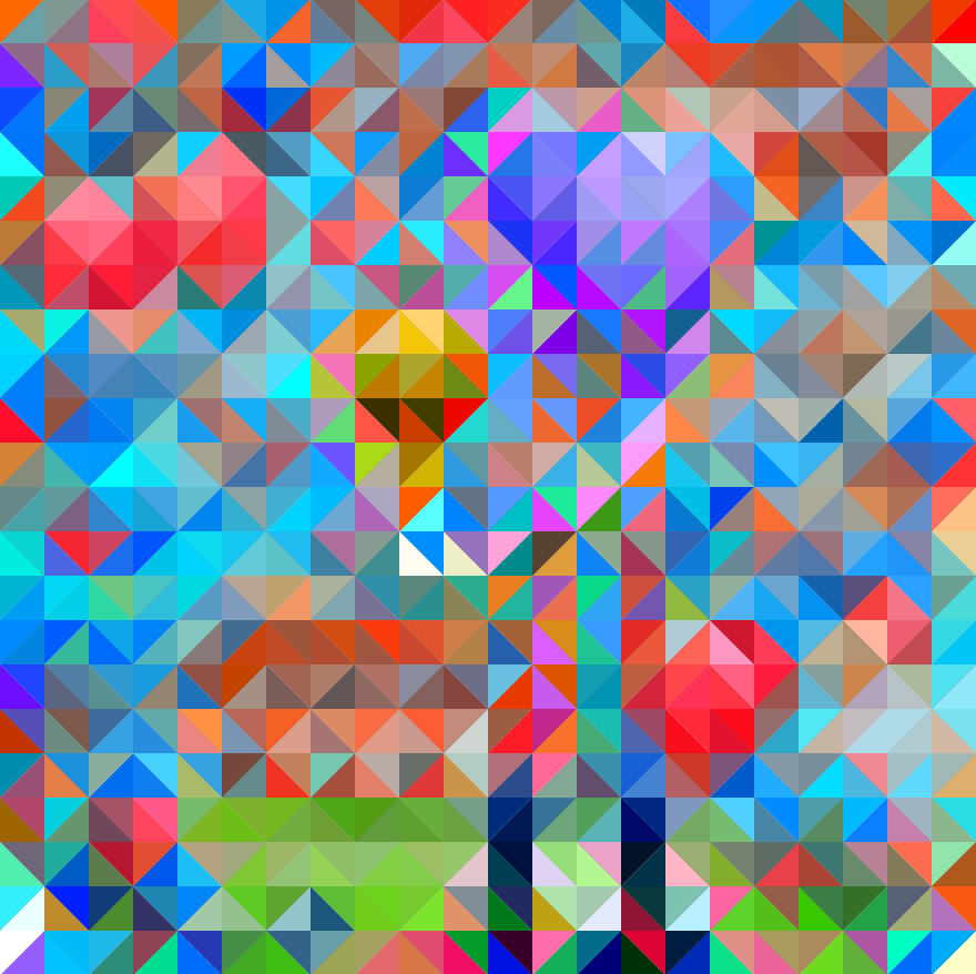
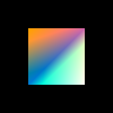
Throughout this process, we introduce and subsequently undo a lot of changes, making the process inefficient and the convergence slow. Another nice approach is to modify only the colors of the triangles rather than their positions and shapes, allowing us to color the mesh structure like a pixel grid:

Prompt = “Balloon” without changing triangle positions

Non-differentiable Operations and the Evolutionary Approach

Up until this point, we’ve only considered gradient descent as a means of solving our central optimization problem. In reality, certain operations involved in this pipeline are not always guaranteed to be differentiable, especially when it comes to rendering. Furthermore, gradient descent optimization narrows the range of images that we’re able to explore. Once a locally optimal solution is found, the optimizer tends to “settle” on it without experimenting further — often to the detriment of the result.

On the other end of the “random-deterministic” spectrum are evolutionary models, which work by introducing random changes at each step. Changes that improve the result are preserved through future steps, whereas superfluous or detrimental changes are discarded. Unlike gradient descent optimization, evolutionary approaches are not guaranteed to improve the result at each step, which makes them considerably slower. However, by exploring a wider set of possible changes to the images, rather than just the changes introduced by gradient descent, we gain the ability to explore more images.

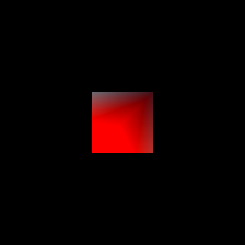
Though we did not tune our evolutionary model to the same extent as our gradient descent optimizer, we were able to produce a version of the program that performs simple tasks such as optimizing with respect to the overall image color.

*Prompt = “red” after 0 and 60 iterations*

3D Shape Optimization

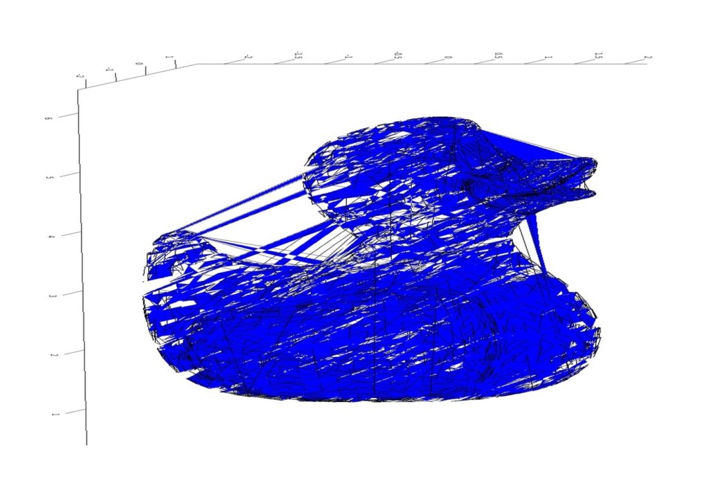
Moving into the third dimension not only gives us a whole new set of geometric primitives to play with, but also introduces fascinating ideas for image augmentations, such as changing the position of the virtual camera. While Nvdiffrast provides a powerful interface for rendering in 3D with automatic differentiation, we quickly discovered that we’d need to implement our own geometric framework before we could test its capabilities.

Nvdiffrast’s renderer is very elegant in its design. It needs only a set of triangles and their indices in addition to a set of vertex colors in order to render a scene. Our first task was to define a set of geometric primitives, as Nvdiffrast doesn’t provide out-of-the-box support for anything but triangles. For anyone familiar with OpenGL, creating an elementary shape such as a sphere is very similar to setting up a VBO/EBO. We set to work creating classes for a sphere, a cylinder, and a cube.

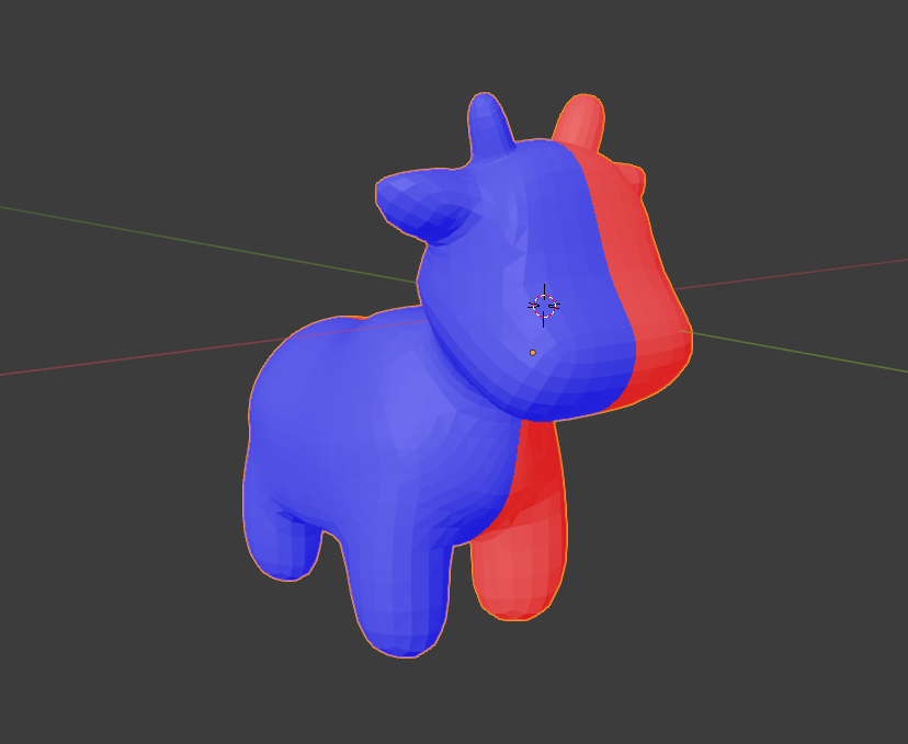
*Random configuration of geometric primitives — a cube, a cylinder, and a sphere — rendered with Nvdiffrast. One example of an input to our algorithm.*

Because the input to Nvdiffrast is one contiguous set of triangles, we also had to design data structures to mark the boundaries between discrete shapes in our triangle list. We did not want the optimizer to operate erratically on individual triangles, potentially breaking up the connectivity of the underlying shape: to this end, we devised a system by which shapes could only be manipulated by a series of standard linear transformations. Specifically, we allowed the optimizer to rotate, scale, and translate shapes at will. We also optimized according to vertex colors as in our previous 2D implementation.

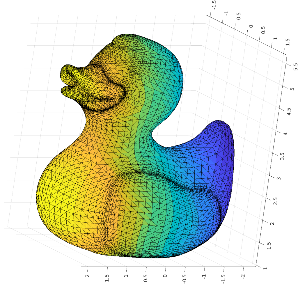
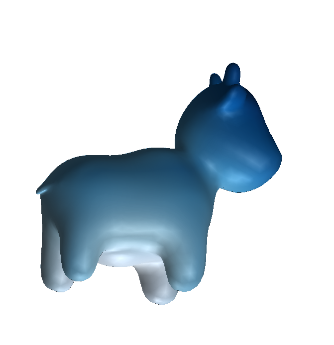
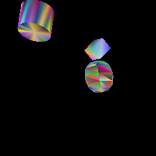
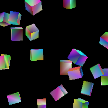
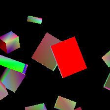
With more time, it would have been great to experiment with new augmentations and learning rates for these parameters: however, setting up a complex environment like Nvdiffrast takes more time than one might expect, and so we have only begun to explore different results at the writing of this blog post. Some features that show promising outcomes are color gradient optimization, as well as the general positioning of shapes:

*prompt = “a centered red squ*are” *(before and after optimization)*

Conclusion

Working on this project over the last few weeks, we saw that it is possible to achieve a lot with neural networks in a relatively short amount of time. Through our exploration of 2D and 3D cases, we were able to generate some early but promising results. More experiments are needed to test the limits of our model, especially with respect to the assembly of complex 3D scenes. Nonetheless, this method of using geometric primitives to synthesize images seems to have great potential, with a number of artistic applications making themselves evident through the results of our work

By SGI fellows Alejandro Pereira and Vivien van Veldhuizen

On the last day of the tutorial week, Nicholas Sharp gave a talk about robustness and debugging in geometry processing. He explained that there are a lot of interesting software tools available for geometry processing, but it is sometimes hard to make these tools robust to different types of data. This is especially true in geometry processing, where there are a lot of different complex data structures such as meshes. Software tools not being robust to different sorts of data, leads to a lot of the available tools becoming unusable, or results coming out wrong. It is therefore important for anyone working with geometry processing, to know what kinds of robustness problems you might encounter and how these may be solved.

Five Common Problems

Nicholas mentioned five of these common problems. The first concerned floating point numbers not being as precise as real mathematical numbers. This could lead to inaccurate data representations, which only pile up as we start computing with the less precise floating point numbers. A second problem to think about was different types of solvers. Nicholas mentioned that we often use numerical solvers in geometry processing, but that some types are a lot more fast and reliable (such as dense linear solvers) than others (for example quadratic or nonlinear solvers). Another common problem Nicholas mentioned was the problem of “bad” meshes. Preloaded meshes could for example have orientation problems, contain overlapping vertices or be nonmanifold. Moreover, even if the meshes were all structured correctly, if we want to run simulations on these meshes, a given algorithm might work on one mesh but not the other. This is because in visual computing, algorithms and inputs (in this case our meshes) are not designed together. Instead, algorithms are just a part of a pipeline and are expected to work on any input data, which is of course not always feasible in practice. Finally, Nicholas briefly talked about machine learning for geometry processing, which is often marketed as an alternative to classic geometry processing. He mentioned that actually, machine learning methods often still contain a lot of geometry processing operations under the hood, so we might still run into any of the problems mentioned above, which might also impact our machine learning results.

To show us what some these problems might look like in practice, Nick gave us two Matlab “puzzles” that we had to solve. Each of these Matlab exercises had some sort of robustness problem and our goal was to find out what these problems were and solve them.

Puzzle 1

In the first exercise, we want to plot a simple mesh. Nothing too complicated right?
Once we have a matrix of vertices V and a matrix for the faces F, it’s just a simple case of running:

>> tsurf(F, V)

However, we get an error:

Error using patch
Value must be of numeric type and greater than 1.

Error in trisurf (line 95)
h = patch('faces',trids,'vertices',[x(:) y(:) z(:)],'facevertexcdata',c(:),...

Error in tsurf (line 132)
t_copy = trisurf(F,V(:,1),V(:,2),V(:,3));

So, what happened? MATLAB told us the error comes from the patch function, so we call patch directly to see what is happening:

>> patches('Faces', F, 'Vertices', V)
Error using patch
Value must be of numeric type and greater than 1.

Because patch only uses V and F, the problem must be in either one of those variables. What if we explicitly give it the X, Y, and Z coordinates of the vertices to plot?


>> patch('XData', V(:,1), 'YData', V(:,2), 'ZData', V(:,3), 'Facecolor', 'Blue')

Yes, progress! We plotted something, and we can see that it is a duck. The vertices matrix seems to be correct, so perhaps i is the faces F that is the problem

Remember the error in the patch function? “Value must be greater than 1.” Well, if you come from a different coding background such as Python, you know that arrays start at index=0. However, this is not the case in MATLAB, where indices start at 1. This means we just need to add 1 to F to fix the problem.

>> F= F+1
>> tsurf(F,V)

Success! We have a lovely duck. Alternatively, we could have used tsurf(F+1,V) and it would also work.

Sometimes error and warnings may be a little intimidating, but if we go step by step from the first error we can find that the source is something as simple as changing a 0 to a 1.

Puzzle 2

For the next exercise, our objective was to compute the geodesic distances along the surface of a ‘meshified’ cow.

For that we will use the 'heat_geodesic' function. In this case, running the function results in the following error:

>> dists = heat_geodesic(V,F,1);
Warning: Matrix is singular, close to singular or badly scaled.
Results may be inaccurate. RCOND = NaN.
> In min_quad_with_fixed/solve (line 409)
In min_quad_with_fixed (line 103)
In heat_geodesic (line 199)

Here the problem is a little more complicated: in our quadratic solver, one of the matrices is singular. This means, among several other equivalent propositions, that the determinant of said matrix is 0.

For now, let’s try to visualize what the mesh looks like using tsurf(F,V):

At first glance, there seems to be nothing wrong. The trick is to realize that some of the vertices in the above mesh are too close to each other. This results in the matrix becoming singular.
One way to solve this is to merge vertices that are closer to a certain threshold. In this case, a threshold of 0.0001 m is enough to remove 120 vertices. The result:

Finally, we get the desired result!

In conclusion: debugging is not only important but also fun! Spending time trying to understand the problem, creating our own hypothesis of what the output should be, and then testing them is what science is all about.