By SGI Fellows Hector Chahuara, Anna Krokhine, and Elshadai Tegegn
During the fourth week of SGI, we continued our work with Professor Paul Kry on Revisiting Computational Caustics. See the “Flat Land Reflection” blog post for a summary of work during week 3, wherein we wrote a flatland program that simulates light reflecting off a surface.
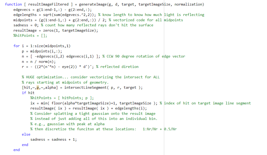
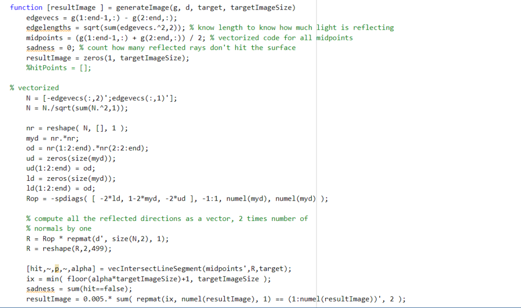
While the flatland program that we wrote did a good job of visualizing the reflection from the source onto the target geometry, the initial code was quite inefficient. It looped over each individual light ray, calculating the reflected direction and intersection with the target one by one. In order to optimize the code, Professor Kry suggested that we try and vectorize the main functions in the program. Vectorizing code means eliminating loops and instead using operations on full vectors and matrices containing the necessary information. In the case of this program, this meant writing a function that simultaneously calculates the intersections of all the reflected rays with the target surface, and then combines them into the resulting image at once (rather than looping over each individual ray’s contribution).
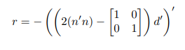
The most challenging part of this task was creating a matrix containing all the reflected directions, rather than just calculating one for a given ray. The equation for the reflected direction from a given normal n is
where d is the direction of the light ray from the source.
We needed to adapt this equation to input a 2xk matrix N containing k normals and get a 2xk matrix R. Because of the n’*n term, this is quadratic in each of the individual columns of N, making vectorization more difficult. One trick we used to resolve this was sparse matrices; that is, matrices with mostly zeros. The idea was that we could calculate and store all the resulting 2×2 matrices from each column in the same large sparse matrix, rather than calculating one at a time. The advantages of this approach is that the sparseness of the matrix makes it less expensive to store, and because other entries are zero, multiplication operations that act on each 2×2 block alone are easy to formulate.
Overall, vectorizing the code was a very fun challenge and good learning opportunity. This project pushed us to apply vectorization to situations with involved and creative solutions.
This blog post was inspired by the talk given by Prof. Yusu Wang during SGI. We use Topological Data Analysis to showcase its feature characterization principles and how it can be used for point cloud surface reconstruction. The code used to generate the different results below are stored on SGI’s GitHub, so give it a try. Let’s go!
Brief Introduction into Persistent Homology
Persistent homology is formed of two words: persistent and homology. Homology comes from homology groups, an intersection between group theory and topology. On a high-level, two objects are homotopic if they can be continuously deformed into one another. As such, they belong to the same group or class because they share the same properties. These homotopy properties can be commonly referred to in examples as the number of holes that an object possesses.
Homology is then used to describe more complex objects such as Simplicial Complexes and Functions.
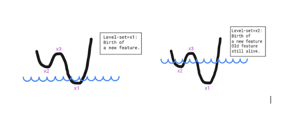
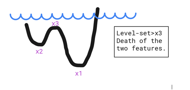
If we take functions, we can map every set level to a property that describes this function. This can best be seen as features induced by local extrema. Local minima tell us that a new feature was born (similar to the hole concept) and the local maxima tell us that some features have been merged and as a result no longer exist. The function below showcases two minima, which means two features are alive at some point simultaneously and disjointly (two separate holes filled water), but will disappear and be merged once the level-set reaches the local maximum.
Features can be seen as local minima that are covered with a level-set.
The death of the features happens when they get merged at a local maximum.
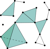
For a set of points, the characterization happens by first constructing a Simplicial Complex (Vietoris-Rips Complex, Čech Complex,…). This follows a logic which connects the points whose circles with radius r centered around them intersect. This is how k-simplices (such as points, edges,triangles, etc. where k is the number of mutually intersecting circles) are built. What happens afterwards is that, in order to find the characteristics of a set of points, the radius r is increased and as we go, the features are detected from the resulting Simplicial Complex.
Now that we have our features, we need to measure their importance and this is what persistence is meant to do. Persistence, is then the act of quantifying the difference between the death and birth of these features, i.e how long a specific feature existed. which helps in assessing the importance of a feature.
For this reason, Persistent Homology can serve as a de-noising tool or can simply act as an object descriptor.
GUDHI: Library for Topological Data Analysis (TDA)
Now, let’s see all of the concepts we have explained in practice. For that, we will use the GUDHI library for Topological Data Analysis.
We present the following examples to showcase the persistence diagrams obtained for different set of points.
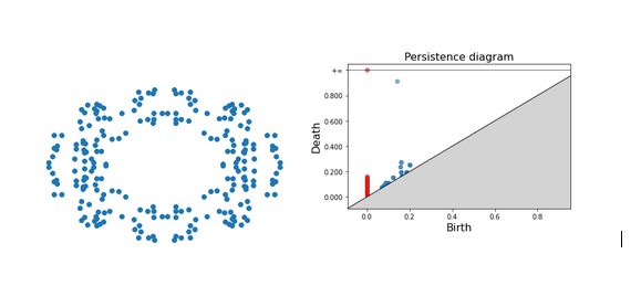
Persistence diagrams have these properties: 1) The red points are the 0-simplices, which are dots, points or disks. 2) The blue points are the 1-simplices characterized by a hole. 3) The points that are far off the diagonal live longer, which means that they are more prominent/important.
For the first example, we can see for instance that one blue dot is very far from the diagonal, which means that this is one of the most important features of our set. The other blue dots which stem from the gap between our points but disappear quickly.
Persistence Diagram of a set of points forming a ring.
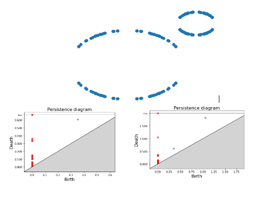
For the second example, we present two persistence diagrams based on two maximum radius thresholds. For a small threshold, we only have one blue dot; the smaller ring is detected because a small threshold matches its small radius. As this threshold gets bigger, we are then able to detect the second bigger ring. Increasing the threshold even further merges these two circles into one component as the different vertices get connected in an indiscernible way.
1) (Left) Persistence Diagram of a set of points forming two rings with a small maximum threshold. 2) (Right) Persistence Diagram of a set of points forming two rings with a big maximum threshold.
Surface Reconstruction with TDA
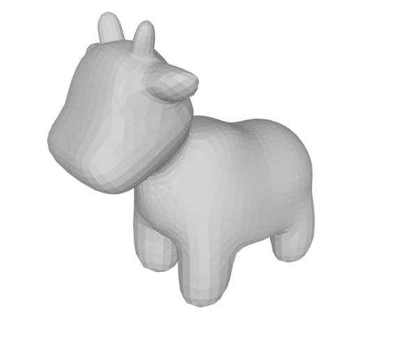
Now that we have used the different elements from the Topological Data Analysis, we will adopt the Simplicial Complex concept and use it to create the surface of a known mesh: spot.
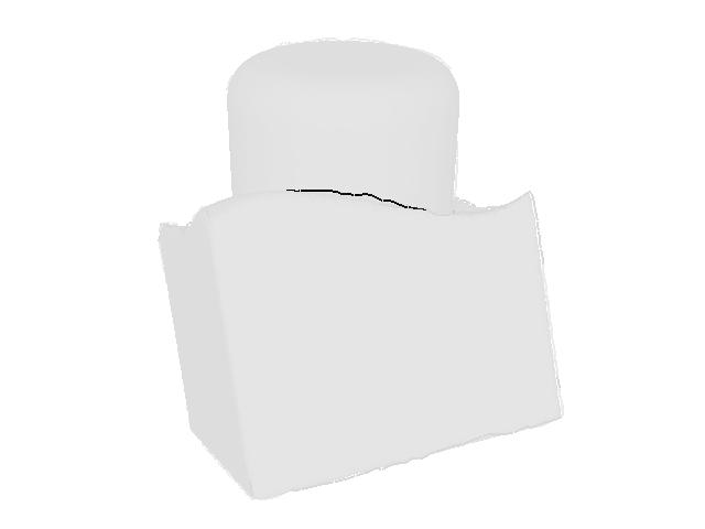
The original mesh.
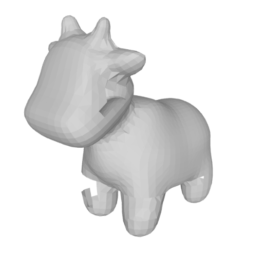
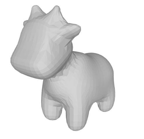
We only consider the point cloud from the mesh and try to estimate the surface by creating the connections between three vertices at once. Once these connections are made, we save a new mesh with these faces connections. Depending on the threshold set to connect the vertices we obtain different levels of precision:
Reconstruction based on the faces from Vietoris-Rips Complex with a low maximum threshold.
Reconstruction based on the faces from Vietoris-Rips Complex with a big maximum threshold.
Conclusion
We have shown in this blog post how Topological Data Analysis and in particular Persistent Homology can be used to find structure in a set of points. This can lead to characterizing the set’s properties in addition to allowing the execution of known tasks in Geometry Processing such as Surface Reconstruction.
References
[1] Persistent Homology—a Survey, Herbert Edelsbrunner and John Harer.
By Tiago De Souza Fernandes, Bryan Dumond, Daniel Scrivener and Vivien van Veldhuizen
If you have been keeping up with some of the recent developments in artificial intelligence, you might have seen AI models that can generate images from a text-based description, such as CLIP or DALL·E. These models are able to generate completely new images from just a single text-prompt (see for example this twitter account). Models such as CLIP and DALL·E operate by embedding text and images in the same vector space, which makes it possible to frame the image synthesis as an optimization problem, ie: find an image that, when processed by a neural network, yields an embedding similar to a corresponding text embedding. A problem with this setup, however, is that it is severely underconstrained: there are many such images and some of them are not very interesting from the perspective of a human. To circumvent this issue, previous research has focused on incorporating priors into this optimization.
Over the last few weeks, our team, under the supervision of Matheus Gadelha from Adobe Research, looked into a specific instance of such constraints: namely, what would happen if the images could only be formed through a simple assembly of geometric primitives (spheres, cuboids, planes, etc)?
An Overview of the Optimization Problem
The ability to unite text and images in the same vector space through neural networks like CLIP lends itself to an intuitive formulation of the problem we’d like to solve: What image comprising a set of geometric primitives is most similar to a given text prompt?
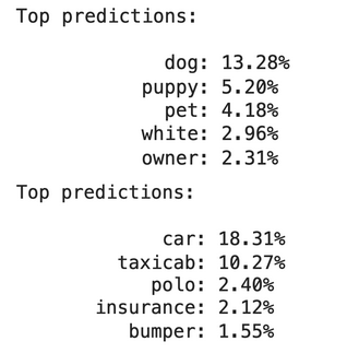
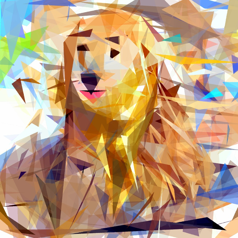
We’ll represent CLIP’s mapping between images/text and vectors as a function, $\phi$. Since CLIP represents text and images alike as n-dimensional vectors, we can measure their similarity in terms of the angle between the two vectors. Assuming that the vectors it generates are normalized, the cosine of the angle between them is simply the dot product \(\langle \phi(Image), \phi(Text) \rangle\). Minimizing this quantity with respect to the image generated from our geometric primitive of choice should yield a locally optimal solution: something that more closely approximates the desired text prompt than its neighbors.
Two sample images — a golden retriever and a 2006 Toyota Camry — alongside their respective descriptions according to CLIP. The cosine similarity of the first image relative to the prompt “a golden retriever” is 0.2690, compared to 0.1586 for the second image.
In order to get a sense of where the solution might exist relative to our starting point, we’d like all operations involved in the process of computing this similarity score to be differentiable. That way, we’ll be able to follow the gradient of the function and use it to update our image at each step. To achieve our goals within a limited two-week timeframe, we desire rasterizers built on simple but powerful frameworks that would allow for as rapid iteration as possible. As such, PyTorch-based differentiable renderers like diffvg (2D) and Nvdiffrast (3D) provide the machinery to relate image embeddings with the parameters used to draw our primitives to the screen: we’ll be making extensive use of both throughout this project.
2D Shape Optimization
We started by looking at the 2D case, taking this paper as our basis. In this paper, the authors propose CLIPDraw: an algorithm that creates drawings from textual input. The authors use a pre-trained CLIP language-image encoder as a metric for maximizing the similarity between the given description and a generated drawing. This idea is similar to what our project hopes to accomplish, with the main difference being that CLIPDraw operates over vector strokes. We tried a couple of methods to make the algorithm more geometrically aware, the first of which is some data augmentations.
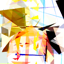
By default, the optimizer has too much creative leeway to interpret which images match our text prompt, leading to some borderline incomprehensible results. Here’s an example of a result that CLIP identifies as a “golden retriever” when left to its own devices:
Prompt = “a golden retriever” after 8400 iterations
Here, the optimizer gets the general color palette right while missing out completely on the geometric features of the image. Fortunately, we can force the optimizer to approach the problem in a more comprehensive manner by “augmenting” (transforming) the output at each step. In our case, we applied four random perspective & crop transformations (as do the authors of CLIPDraw) and a grayscale transformation at each step. This forces the optimizer to imitate human perception in the sense that it must identify the same object when viewed under different ambient conditions.
Fortunately, the introduction of data augmentations produced near-instant improvements in our results! Here is a taste of what the neural network can generate using triangles:
Prompt = “a Golden Retriever”Prompt = “a lighthouse”
Generating Meshes
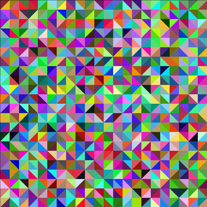
In addition to manipulating individual shapes, we also tried to generate 2D triangular meshes using CLIP and diffvg. Since diffvg doesn’t provide automatic support for meshes, we circumvented this problem using our own implementation where individual triangles are connected to form a mesh. We started our algorithm with a simple uniform randomly-colored triangulation:
Initial mesh
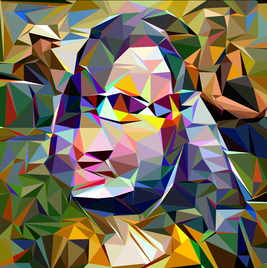
Simply following each step in the gradient direction could change their positions individually, destroying the mesh structure. So, at each iteration, we merge together vertices that would have been pushed away from each other. We also prevent triangles from “flipping”, or changing orientation in such a way that would produce an intersection with another existing triangle. Two of the results can be seen below:
Prompt = “Monalisa”Prompt = “Batman”
Throughout this process, we introduce and subsequently undo a lot of changes, making the process inefficient and the convergence slow. Another nice approach is to modify only the colors of the triangles rather than their positions and shapes, allowing us to color the mesh structure like a pixel grid:
Prompt = “Balloon” without changing triangle positions
Non-differentiable Operations and the Evolutionary Approach
Up until this point, we’ve only considered gradient descent as a means of solving our central optimization problem. In reality, certain operations involved in this pipeline are not always guaranteed to be differentiable, especially when it comes to rendering. Furthermore, gradient descent optimization narrows the range of images that we’re able to explore. Once a locally optimal solution is found, the optimizer tends to “settle” on it without experimenting further — often to the detriment of the result.
On the other end of the “random-deterministic” spectrum are evolutionary models, which work by introducing random changes at each step. Changes that improve the result are preserved through future steps, whereas superfluous or detrimental changes are discarded. Unlike gradient descent optimization, evolutionary approaches are not guaranteed to improve the result at each step, which makes them considerably slower. However, by exploring a wider set of possible changes to the images, rather than just the changes introduced by gradient descent, we gain the ability to explore more images.
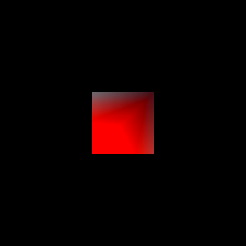
Though we did not tune our evolutionary model to the same extent as our gradient descent optimizer, we were able to produce a version of the program that performs simple tasks such as optimizing with respect to the overall image color.
Prompt = “red” after 0 and 60 iterations
3D Shape Optimization
Moving into the third dimension not only gives us a whole new set of geometric primitives to play with, but also introduces fascinating ideas for image augmentations, such as changing the position of the virtual camera. While Nvdiffrast provides a powerful interface for rendering in 3D with automatic differentiation, we quickly discovered that we’d need to implement our own geometric framework before we could test its capabilities.
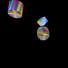
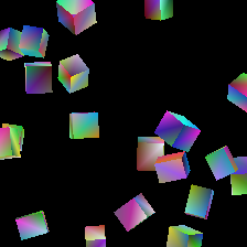
Nvdiffrast’s renderer is very elegant in its design. It needs only a set of triangles and their indices in addition to a set of vertex colors in order to render a scene. Our first task was to define a set of geometric primitives, as Nvdiffrast doesn’t provide out-of-the-box support for anything but triangles. For anyone familiar with OpenGL, creating an elementary shape such as a sphere is very similar to setting up a VBO/EBO. We set to work creating classes for a sphere, a cylinder, and a cube.
Random configuration of geometric primitives — a cube, a cylinder, and a sphere — rendered with Nvdiffrast. One example of an input to our algorithm.
Because the input to Nvdiffrast is one contiguous set of triangles, we also had to design data structures to mark the boundaries between discrete shapes in our triangle list. We did not want the optimizer to operate erratically on individual triangles, potentially breaking up the connectivity of the underlying shape: to this end, we devised a system by which shapes could only be manipulated by a series of standard linear transformations. Specifically, we allowed the optimizer to rotate, scale, and translate shapes at will. We also optimized according to vertex colors as in our previous 2D implementation.
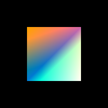
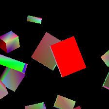
With more time, it would have been great to experiment with new augmentations and learning rates for these parameters: however, setting up a complex environment like Nvdiffrast takes more time than one might expect, and so we have only begun to explore different results at the writing of this blog post. Some features that show promising outcomes are color gradient optimization, as well as the general positioning of shapes:
Prompt = “red”Prompt = “rainbow”prompt = “a centered red square” (before and after optimization)
Conclusion
Working on this project over the last few weeks, we saw that it is possible to achieve a lot with neural networks in a relatively short amount of time. Through our exploration of 2D and 3D cases, we were able to generate some early but promising results. More experiments are needed to test the limits of our model, especially with respect to the assembly of complex 3D scenes. Nonetheless, this method of using geometric primitives to synthesize images seems to have great potential, with a number of artistic applications making themselves evident through the results of our work
By Caroline Huber, Alan Goldfarb, and Denisse Garnica
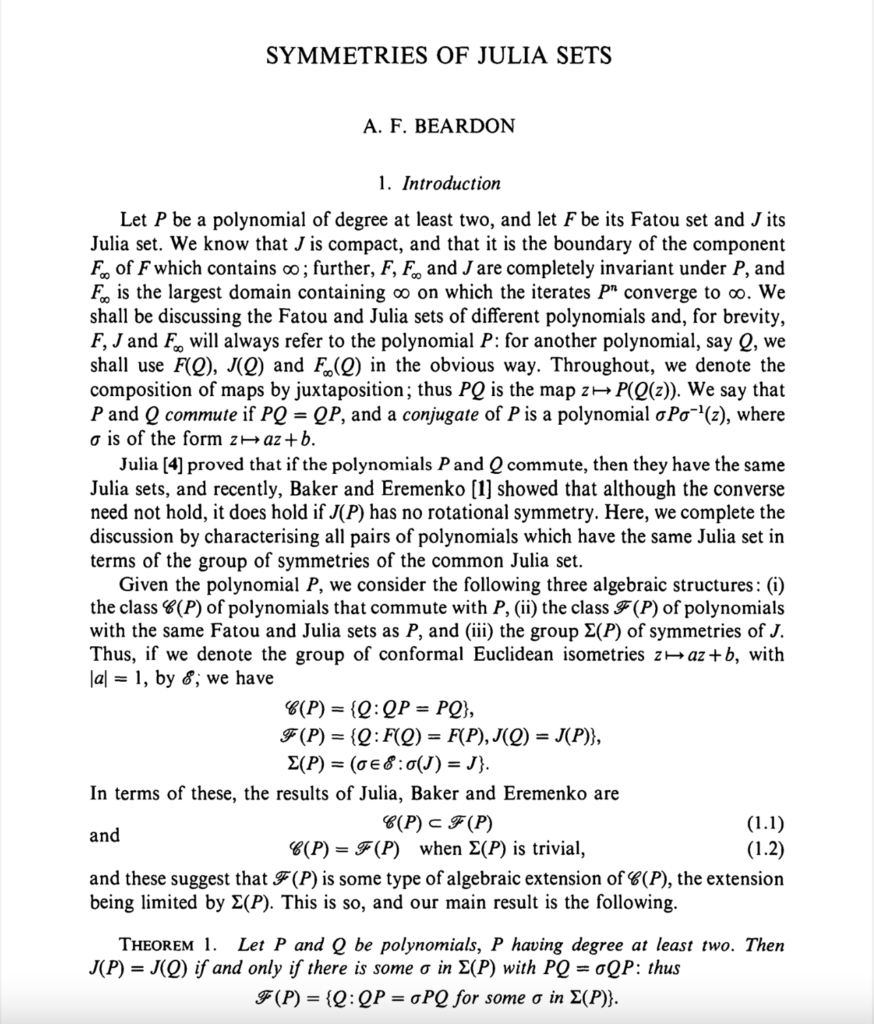
In the first project of SGI, for us, Julia Sets – where we (in simple terms) attempt to approximate 2D and 3D shapes with a Julia Set – much interesting work was done. The official problem statement is: Can we train a neural network to predict the corresponding filled Julia set approximation for any given input shape? With daily collaborative meetings and independent coding work we first attempted to understand how to construct these sets with code. We worked our way through several established papers on the subject both independently as well as in several collaborative zooms (see pdfs below).
Then, we worked on experimenting with some base code that one of our mentors, Richard Liu, provided. By experimenting, we mean that we altered various attributes of the presented function and observed the effects on the fractal output. We changed the values of the roots, their multiplicities, the number of roots, and we added scalar multiples and so on. For reference, Figure 1 is the original fractal. Multiplying by a scalar less than one resulted in less separation between the affected roots (closer together). This is shown in the following figures: multiplying the whole function by a scalar of 0.5 resulted in figure 2 and multiplying just the second and fourth roots by a scalar multiple of 0.5 resulted in figure 3.
Figure 1Figure 2Figure 3
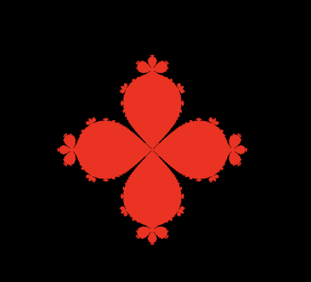
Conversely, multiplying by a scalar larger than 1 resulted in increased separation between the affected roots (farther apart). The result of multiplying by a scalar of 1.3 resulted in figure 4.
Figure 4Figure 5Figure 6
Further experimentation included scalar multiple and changing all roots to be double (multiplicity 2), as seen in figure 5, and scalar multiple with only changing the multiplicity of a single root (to be double), as seen in figure 6.
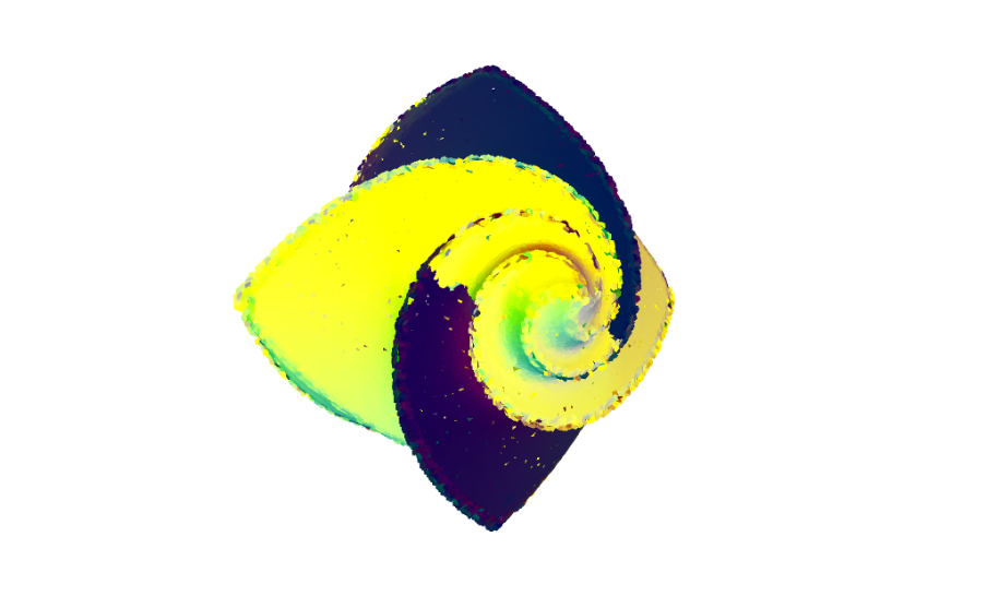
We created a function to add color to the non-Julia Set points. Defining the color with the “escape velocity”. The Julia set -explained in a very ambiguous way- is a set of points that stays in some certain region after many iterations of a function. The “escape velocity” is how long it takes to a point to go outside the region. According to that number we change the color of the point. And we obtain images like this one.
Here all the black points represent the Julia set. The dark-green points are the ones that have a minor escape velocity and the brightest are the ones that took longer to go outside.
We decided that it would be helpful to be able to zoom into these fractals and see what they look like up close (especially with the alterations). So, we added code that zoomed in on a point slightly off-center. Then, we combined several of those images into a gif that runs through them all. (see attachment 1)
Attachment 1
We collaborated to create another gif that runs through frames where the root location is altered, and the picture zooms in on this change. We provided the code to identify and alter the roots and then combined the frames. (see attachment 2 for altered root multiplicities and attachment 3 for a zoom of altered roots).
Attachment 2Attachment 3
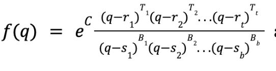
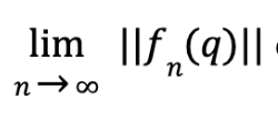
Now that Julia sets have been seen in an intuitive way, let’s see a little more formality. Julia sets of rational maps are determined as follows: Given a rational map (a function of the form f(q)) a complex number q is in the corresponding Julia set if the below limit does not diverge. Here, fn denotes the nth recursion of f. The constants r1,r2, . . ., rt and s1, s2 , . . .,sb are respectively called the top and bottom roots of f.
Equation 1Equation 2
In order to generate plots of these sets we approximated the set by iterating the function a fixed number of times and comparing the output against a threshold value. Only inputs which produced a value below the threshold were included in the Julia set. We then plotted the filled Julia set by plotting the interior of the Julia set.
Some of the filled Julia sets we generated behaved in ways which differed from our initial expectations. According to a paper by Dr. Theodore Kim, points close enough to top roots would be included in the filled Julia set and points close enough to bottom roots would not. Dr. Kim stated that to approximate a given curve with a Julia set one should use a rational function with roots along that curve. However, we realized that symmetric placement of the roots can generate asymmetric Julia sets and that placing roots along the boundary of a shape did not always produce a filled Julia set corresponding to that shape.
In order to get a better understanding of why this might be occurring, we read a few papers describing the mathematical structure of Julia sets of rational functions. We delved deeper into these papers and explained some strange properties about Julia sets. For instance, a Julia set of a polynomial cannot have any mirror symmetries which are not also rotational symmetries. This is the case even if the placement of the roots is symmetric. This led us to the realization that adding roots to a function can have global consequences on the shape of the function’s Julia set which makes the problem of approximating even simple shapes with Julia sets seem more difficult than initially anticipated.
This project has been very interesting for the three of us and we are looking forward to see what we can achieve in the future. We will continue exploring Julia sets, and hopefully we will be able to approximate interesting figures!
By Abraham Kassahun, Dimitry Kachkovski, Hongcheng Song, Shaimaa Monem
Introduction
It has been two weeks of the projects phase in SGI and our team has been working under the guidance of David Levin and Rohan Sawhney on a very interesting approach to solving differential equations using Mixed Finite Element Method.
In the beginning we were looking at how general Finite Element Methods (FEM) are used to solve the 2D Screened Poisson Equation (and later on a 3D one). First and foremost, we need to understand what FEM is. It is a discretization method that allows us to accurately solve differential equations. It allows us to break up a large system into simpler finite parts (in our case – triangles), and to make certain assumptions over these finite elements that help find a feasible solution.
If we look into the very simple case of only one triangle mesh, then given 3 vertices \(v_1, v_2, v_3\) that form this triangle, we attach a value of a function \(u\) at each of them (that is \(u(\textbf{v}_1),u(\textbf{v}_2),u(\textbf{v}_3)\)are known). To get the value of \(u(\textbf{v})\), for a point \(\textbf{v}\) inside the triangle, we can use various ways of interpolating between the 3 given values. Linear interpolations are often very useful for simulation, and we can use for instance barycentric coordinates as a way to interpolate these values.
A variation of the FEM method that we are exploring is called Mixed FEM. Its main idea is the introduction of supplementary independent variables that create additional constraints on the system. Mixed finite element method can precisely solve some very complex PDEs, while the ultimate goal of utilizing it in our project is to provide another more flexible skinning strategy, which automatically tunes deformation parameters to triangles by artist specified controls, while paving the way to an optimized version of the solver via the Adjoint Method.
Screened Poisson Equation
Figure 1. Screened Poisson equation solve over a 2D mesh with animated alpha parameter. (Credit: Abraham Kassahun Negash)
To understand how mixed FEM works, we first applied it to the heat equation. It turns out that it doesn’t have any advantages when applied to the heat equation, but it was a good pedagogical detour to understand how it works exactly. The heat equation is a type of Poisson equation described as:$$\Delta u = f$$ If solved as is, the resulting equation will not have a unique solution due to the absence of a Dirichlet boundary condition. Instead we modified the equation slightly by including an \(\alpha u\) term which allows the equation to be solved without explicitly giving any boundary conditions in MATLAB. $$\Delta u – \alpha u = f$$ This equation is also called the screened Poisson equation. We can solve for \(u\) by minimizing the following energy. $$E(u) = \frac{1}{2}\int_{\Omega}||\nabla u||^2 \,d\Omega + \frac{1}{2}\int_{\Omega} \alpha ||u||^2 \,d\Omega – \int_{\Omega} fu \,d\Omega$$ Where \(\Omega\) is our domain of interest. We can define \(u\) as a vector of values evaluated at the vertices of a triangle mesh. Then the equation can be discretized by writing \(u\) as the weighted average of vertex values. $$u(x) = \sum_{i=1}^3{\phi_i (x) u_i}$$ Where \(\phi_i (x)\) are the shape functions we use to interpolate \(u\) inside the triangle. We are going to let \(u\) be piecewise linear over our mesh by choosing linear shape functions. Thus the gradient of \(\phi\) is constant inside the triangle. Substituting into \(u\) and performing the integration we get the following expression. $$E(u) = \frac{1}{2}u^T G^T W G u + \frac{1}{2}\alpha u^T M u – u^T M f$$ Where:
\(G\) is the gradient matrix defined over the mesh
\(W\) is the weight matrix resulting from integrating \(\nabla u\) over faces
\(M\) is the mass matrix resulting from integrating functions over vertices
\(G\) is the gradient operator over the mesh and only depends on the vertex positions. The mass and weight matrices can be taken as identity by assuming a uniform mesh of equal triangles. It can be seen that the term with an \(\alpha\) acts the potential energy of a spring penalizing deviation of \(u\) from 0, thus preventing the solution from blowing up. The solution therefore reduces to $$E(u) = \frac{1}{2}u^T G^T G u + \frac{1}{2}\alpha u^T u – u^T f$$
To solve for \(u\) we formulate an optimization problem in a discrete form over some finite cells of a given surface, that is we build a Finite Element system and find the minimizer as follows:
$$u^* = \arg \min_{u}(\frac{1}{2} u^T G^T G u + \frac{1}{2} \alpha u^T u – u^T f)$$
Finally, to minimize the above system with the standard FEM, we must take the derivative of the function w.r.t. \(u\), and since the system is quadratic, setting the result to zero and solving for \(u\) will yield the answer. That is if we define the energy as $$E(u)=\frac{1}{2}u^T G^T G u + \frac{1}{2}\alpha u^T u – u^T f)$$ then we compute the gradient $$\nabla_u{E}=G^T G u + \alpha u – f =0$$ and we get $$G^T G u + \alpha u = f\\ (G^T G + \alpha I)u=f\\ u=(G^T G + \alpha I)^{-1} f$$
This means that the discrete solution can be computed through a linear system solution.
Mixed FEM
Figure 2. Mixed FEM solution of the ARAP energy by rotating a single triangle. (Credit: Shaimaa Monem)
As mentioned in the introduction, the main idea behind Mixed FEM is to introduce an additional independent variable that we solve for to allow us to optimize the search for the full solution to our system. That is, we will make everything much more complicated so as to make it easier later on! Yay!
We introduce such a variable by taking a part of the original energy equation \(E(u)\), and setting a constraint. That is, we want to reformulate the original minimization as $$g^*,u^* = \arg \min_{u,g}(\frac{1}{2} g^T g + \frac{1}{2} \alpha u^T u – u^T f)\\ s.t. \ Gu-g=0$$
The idea definitely feels awkward at first. But what we are looking to do is to define \(Gu\) as some variable that is independent of \(u\) itself, but that constrains the system for \(u\). Think of how the search for \(u\) was like turning some dials, and \(Gu\) was another dial that would turn as you try different settings for \(u\). Our goal is to separate that connection so that we can search for both independently, with that search governed by the established rule aka. our constraint.
To solve the newly emergent constrained optimization we use the method of Lagrange Multipliers and formulate our system as: $$\mathcal{L}{g^*,u^*,\lambda}=\arg \max_{\lambda} \min_{g^*,u^*}E + \lambda^T(Gu-g)\\ \mathcal{L}{g^*,u^*,\lambda}=\arg \max_{\lambda} \min_{g^*,u^*} \frac{1}{2} g^T g + \frac{1}{2} \alpha u^T u – u^T f + \lambda^T(Gu-g) $$
Now, we just need to take the gradient w.r.t. each of the variables, set them as before to 0, and solve for our 3 variables! That gets us: $$ \nabla_g=g-\lambda=0\\ \nabla_u=\alpha u – f + G^T \lambda=0\\ \nabla_{\lambda}=Gu-g=0$$
These 3 conditions that we got are known as Karush-Kuhn-Tucker (KKT) conditions. Using them we formulate a larger system that we solve: $$\begin{bmatrix} I & 0 & -I \\ 0 & \alpha I & G^T \\ -I & G & 0 \end{bmatrix} \begin{bmatrix} g\\ x\\ \lambda \end{bmatrix} = \begin{bmatrix} 0\\ f\\ 0 \end{bmatrix}$$
Solving this system will give us the solution that we are after.
Now this alone is obviously not a way to speed our solution up. However, the Mixed FEM formulation allows us to combine it with a numerical method known as the Adjoint Method, which in turn will indeed speed up the whole system. It also allows us to leverage certain aspects of deformation energies and their formulations which avoids such heavy handed computations as SVDs.
But before we get there, let’s move away from the toy problem, and consider how our mesh will deform.
As-Rigid-As-Possible (ARAP) Energy
Figure 3. A sine-based animation using Automatic Skinning using Mixed FEM. (Credit: Dimitry Kachkovski)
Deformation of elastic objects can be described using various different models. The one we consider is known as the As-Rigid-As-Possible model (Sorkine and Alexa, 2007).
ARAP is a powerful energy term which is invariant to rigid transformations, and it is designed to measure deformation in our system setting clearly, which has the form: $$E(F) = \| S – I \|_{F}^2$$ Where \(F\) represents the total transformation while \(S\) is a parameter unrelated to rigid transformation, which can be generated from polar decomposition from \(F\) using the relation \(F = RS\), where \(R\) is a rigid transformation. Therefore, energy is only dependent on non-rigid transformation, which has a global minimum at Identity. In this case, \(E(R) = 0\) and \(E(RS) = E(S)\). Instead of finding \(S\) through decomposition every time, what Mixed FEM allows us to do is to let \(S\) be an independent variable and enforce the relation \(F = RS\) with a constraint. Therefore, \(E\) can now be written as:$$E(S) = \| S – I \|_{F}^2$$
Using second-order Taylor expansion, ARAP energy takes the following form: $$E(S) = \frac{1}{2}S^THS + G^TS$$Where \(H\) and \(G\) are Hessian and gradient matrices, respectively.
Any rigid transformation exerted on triangle mesh will result in zero ARAP energy, but for any non-rigid deformation on triangle mesh, ARAP will clearly generate the corresponding energy. For example, in our gingerBrad man example, we pin down a rotation for a triangle; hence, the only possible situation to keep ARAP energy be zero is forcing all rotations of other triangles to be the same as the pinned one. You can imagine that if one of those triangles does not conform to the same rotation, non-rigid deformation will be generated in that triangle, leading to the growth of ARAP energy. So, ARAP skinning energy is indeed measuring the difference of energy between the current system state and the As-Rigid-As-Possible state with two boundary conditions, and the current state will finally reach the As-Rigid-As-Possible state by the optimizer.
Yoga Performance with Adjoint Method
1.1 Motivation and task formulation
Assuming we have a physics-based animation scene that we would love to visualize, we always start from a the continuous setting, then we choose a discretization scheme that allows us to write a piece of code to simulate our animations, we then pick our favorite programming language and turn the discrete model into a script that our computers can understand and deal with. If we are animating a character, then we would like it to match a specific behavior that is visually appealing, for example a special yoga pose. Well, assuming our character is sportive and flexible, then our simulator might do a good job imitating the desired behavior, if we define flexibility and athletic ability as parameters and feed them to our model. And we can see that in order to achieve successful animation we required three ingredients:
Discrete model simulating our object’s animations,
Target behavior for the object,
Input parameters tuning the object’s properties.
Sounds simple enough! But it implies that we need to know everything beforehand, which is not the case with movie character animation. We might know our target behavior but we do not know the parameters values that take us to this specified behavior, for instance how do we tune flexibility for gingerBrad so that it can do yoga without breaking?
We can express this yoga pose as a desired deformation through a deformation energy which happens to be the well known and previously mentioned ARAP energy. Therefore, we can basically translate this into an optimization task to find, for instance, the threshold \(p^{\star}\) of the flexibility parameter that is enough to reach the yoga pose, $$p^{\star} = \arg \min_{p} \ E_{ARAP}(p)$$
If you have been to a yoga class, then you have heard your instructor say – “Keep your toes forward and your heels down to the floor, straight back…” – and so on! Well, this is one of the powers that comes with using skinning technique: we can easily pin gingerBrad’s feet to the ground using handles, as follows: $$p^{\star} , x^{\star} = \arg \min_{p,x} \ E_{ARAP}(p) + \frac{k}{2} \| P x – x_{pinned} \|^2 $$
This means that we can optimize not only over \(p\) but also over all vertex positions \(x\) of the gingerBrad mesh, and we get \(x^{\star}\) the optimal position that is as close as possible to the pose we want, with heals \(x_{pinned}\) pinned to the ground. In the equation above \(P\) is a pinning matrix that selects from \(x\) only the verts to which we assign boundary conditions (here simply pinning!).
So far so good. Now let us imagine a more complex scenario where it is hard to exactly define what that target pose would look like. To picture this situation, let us assume that the gingerBrad character actually got a job as a yoga instructor, and now many characters are standing behind copying the yoga moves! Well, realistic experience tells us that they will not all reach the same exact final yoga pose, as they have different body properties reflected through a wide range of flexibility parameter values, and for the sake of our health and sanity we want to avoid solving a separate problem for each participant, especially ifgingerBrad is a very beloved famous coach and his class is always full :-)
We know that we want all of them to go as close as they could to a specific yoga pose, so let us assume, for simplicity, that we want them to rotate their bodies while still standing on the ground We can represent this very special yoga pose with a rotation matrix \(R\). But we can clearly see that the way this rotation task goes for each of them depends on their shapes, i.e. positions \(x\), and properties, or, as we call it, parameters \(p\), which in turn depend on the assigned rotation, meaning we have \(x(R)\) and \(p(R)\).
To find the rotation that each of them can achieve, we must formulate another optimization task:
$$ R^{\star} = \arg \min_{R} \ E_{ARAP}(p) + \frac{k}{2} \| P x – x_{pinned} \|^2 + \| R – R_{pinned} \|^2$$
Where \(R_{pinned}\) makes sure that our animated characters perform rotation around their pinned vertices, for consistency.
Now arises a huge EXISTENTIAL QUESTION, if \(R\) depends on\(p\) and \(x\) which in return are functions of \(R\), how can we compute any of them??
1.2 Apply Adjoint Method
Well basically the adjoint method is the solution to this problem, and we will go through this step by step.
First, remember that finding \(R^{\star}\) is our ultimate goal, as we want to visualize the yoga poses for all our animated characters and visualize how they perform. We ask ourselves, what do we need to solve the second optimization to compute \(R^{\star}\)? And the simple answer is that we need to find the critical points to the gradient $$E(R)= E_{ARAP}(p)+ \frac{k}{2} \| P x – x_{pinned} \|^2 + \| R – R_{pinned} \|^2\\ \frac{d E(R)}{d R} = \frac{\partial x}{\partial R} \frac{\partial E(R)}{\partial x} + \frac{\partial p}{\partial R} \frac{\partial E(R)}{\partial p} + \frac{\partial E(R)}{\partial R} = 0$$ While computing this gradient requires \(\frac{\partial x}{\partial R}\) and \(\frac{\partial p}{\partial R}\) as \(x\) and \(p\) are functions of \(R\).
Second, we can actually exploit the first optimization problem to compute \(\frac{\partial x}{\partial R}\) and \(\frac{\partial p}{\partial R} \).
Let’s perform the steps for a special parameter and explain more. We want \(p\) to relate to the deformation \(F\) which expresses the deformed state. We can specifically use the polar decomposition and write \(F\) as a decomposition of a rotation matrix \(R\) and a symmetric matrix \(S\), i.e. \(F = R S\). Remember that we are optimizing \(R\), therefore we are left with \(S\) to pick as our parameter. Moreover, we can find a linear operator called deformation gradient \(B\) that represents this deformation and basically takes our character from its rest reference pose to the deformed yoga performance pose. This gives us a constraint \( B x = RS\) which leads to the following constrained optimization problem
$$ S^{\star} , x^{\star} = \arg \min_{S,x} \ E_{ARAP}(S) + \frac{k}{2} \| P x – x_{pinned} \|^2 $$
Such that \( B x = R S\) (note: I am skipping technical details for simplicity!)
Now the latest constrained optimization task can be happily solved through a Lagrangian energy, actually arising from a mixed FEM problem as explained previously.
$$L(S, x, \lambda) = E_{ARAP}(S) + \frac{k}{2} \| P x – x_{pinned} \|^2 + \lambda (Bx – RS)$$
And like we saw in the very beginning of the report we proceed with computing the gradients of \(L(S, x, \lambda)\) w.r.t. its three different variables and formulate a linear system to solve
$$\nabla_S L = HS + g^T – R^T \lambda = 0\\ \nabla_x L = \frac{k}{2} P^TP + B^T \lambda = 0\\ \nabla_{\lambda} L = B x- R S = 0$$
We rewrite this as \(A y = b \) , where \(A\) is the KKT matrix and \(y = (S^{\star}, x^{\star} , \lambda)^T\) is the solution for our first optimization problem.
Third, we can extract \(S^{\star}\) and \(x^{\star}\) from \(y\) and fix them in \(E(R)\), which leads to $$E(R)= E_{ARAP}(S^{\star})+ \frac{k}{2} \| P x^{\star} – x_{pinned} \|^2 + \| R – R_{pinned} \|^2$$
Fourth, now we can see that, actually, the derivatives that we require are \(\frac{\partial x^{\star}}{\partial R}\) and \(\frac{\partial S^{\star}}{\partial R}\) , which can be computed by differentiating \(y\) , i.e. \(\frac{\partial y}{\partial R} = (\frac{\partial S^{\star}}{\partial R} , \frac{\partial x^{\star}}{\partial R} , 0)^T\), given by $$\frac{\partial y}{\partial R} = \frac{\partial A^{-1}}{\partial R} \ b\\ \frac{\partial y}{\partial R} = – A^{-1 } \ \frac{\partial A}{\partial R} A^{-1 } \ b$$
Finally, now that we have \(\frac{\partial x^{\star}}{\partial R}\) and \(\frac{\partial S^{\star}}{\partial R}\), we can basically substitute them into the energy derivative \(\frac{d E(R)}{d R}\) and find \(R\) as the critical point, Woooh!
One more important aspect that we need to take care of is to make sure that \(R\) stays still as a rotation matrix along the optimization task, for this reason, we explicitly write \(R\) as an orthogonal 2D matrix $$R(\theta) = \begin{bmatrix} cos \theta & sin \theta \\ – sin \theta & cos \theta \end{bmatrix} $$ And express our energy in terms of \(\theta\) instead, as follows $$\frac{d E(\theta)}{d \theta} = \frac{\partial x}{\partial \theta} \frac{\partial E(x(\theta),p(\theta),\theta)}{\partial x} + \frac{\partial p}{\partial \theta} \frac{\partial E(x(\theta),p(\theta),\theta)}{\partial p} + \frac{\partial E(x(\theta),p(\theta),\theta)}{\partial \theta} = 0$$
All that is left is to give the solver of our choice an initial guess of the angle and let it run. And now we can find the yoga poses for all participants in the yoga class coached by gingerBread and render an animation if we want.
Figure 4. Manipulation of handles with Automatic Skinning using Mixed FEM. (Credit: Hongcheng Song)
Take away home: next time you go to Yoga class do not forget your Adjoint Method 🙂
1.3 Apply Adjoint Method to High Resolution Mesh
Even though the adjoint method is able to accelerate the optimization process of angles by analytical gradient, it is still an extremely expensive process to use for high resolution meshes. Therefore, we use average biharmonic weights and optimized angles of blue noise sample points to approximate the final result. This approximation propagates those optimal solutions to all triangles by introducing biharmonic weights, allowing a smooth angle interpolation across the surface and reducing enormous calculation expenses required for optimizing all triangles.
Where \(f\) is the number of triangle faces, \(h\) is the number of sample points. \(W_{i, j}\) is the biharmonic weights of a triangle with respect to each sample point, and \(\theta_j\) is the optimized solution of sample points.
References (APA style):
Sorkine, O., & Alexa, M. (2007, July). As-rigid-as-possible surface modeling. In Symposium on Geometry processing(Vol. 4, pp. 109-116).
By SGI Fellows Hector Chahuara, Anna Krokhine, and Elshadai Tegegn
During the third week of SGI, under the guidance of Associate Professor Paul Kry, we worked on Revisiting Computational Caustics. The team returned to this project by EPFL, exploring ideas in differentiable rendering and alternative solutions for optimal transport.
The shape of a mirror can be designed such that the reflection of sunlight on the surface forms a desired image on an adjacent wall.
The project’s starting point was designing a simple flat land that isn’t completely flat as a reflective surface. By changing the reflective land’s surface from flat to something that resembles a zigzag, by a little amount each time, we were able to notice it impacts the reflected rays a lot more and disperses them all around the surface.
We first designed the light source with the light rays (color red), and the reflective surface (color green), and the final surface (color light blue) we wanted to project our light rays. Then our simulation began by varying the reflective surface with the function by \(t\); for \(t\) from 0 to 0.005 with 100 line spaces.
\(f(x) = \sin(8x)\cdot t\), for \(x\): -1 to 1.3 with 100 linespaces
Since we multiply the function by \(t=0\) at the first iteration, the reflective surface is a flatland. But as t increases, through every iteration, the reflective becomes more like a \(\sin x\) function, giving us light rays that are spread across the final surface.
By SGI Fellows Xinwen Ding, Josue Perez, and Elshadai Tegegn
During the second week of SGI, we worked under the guidance of Prof. Yusuf Sahillioğlu to detect planes and edges from a given point cloud. The main tool we applied to complete this task is the Random Sample Consensus (RANSAC) algorithm.
Definition
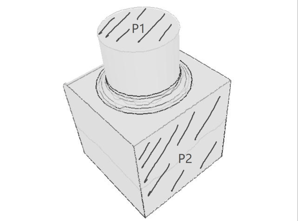
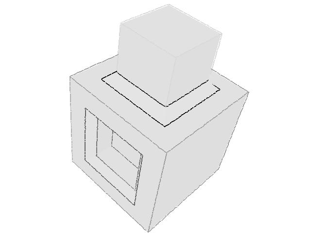
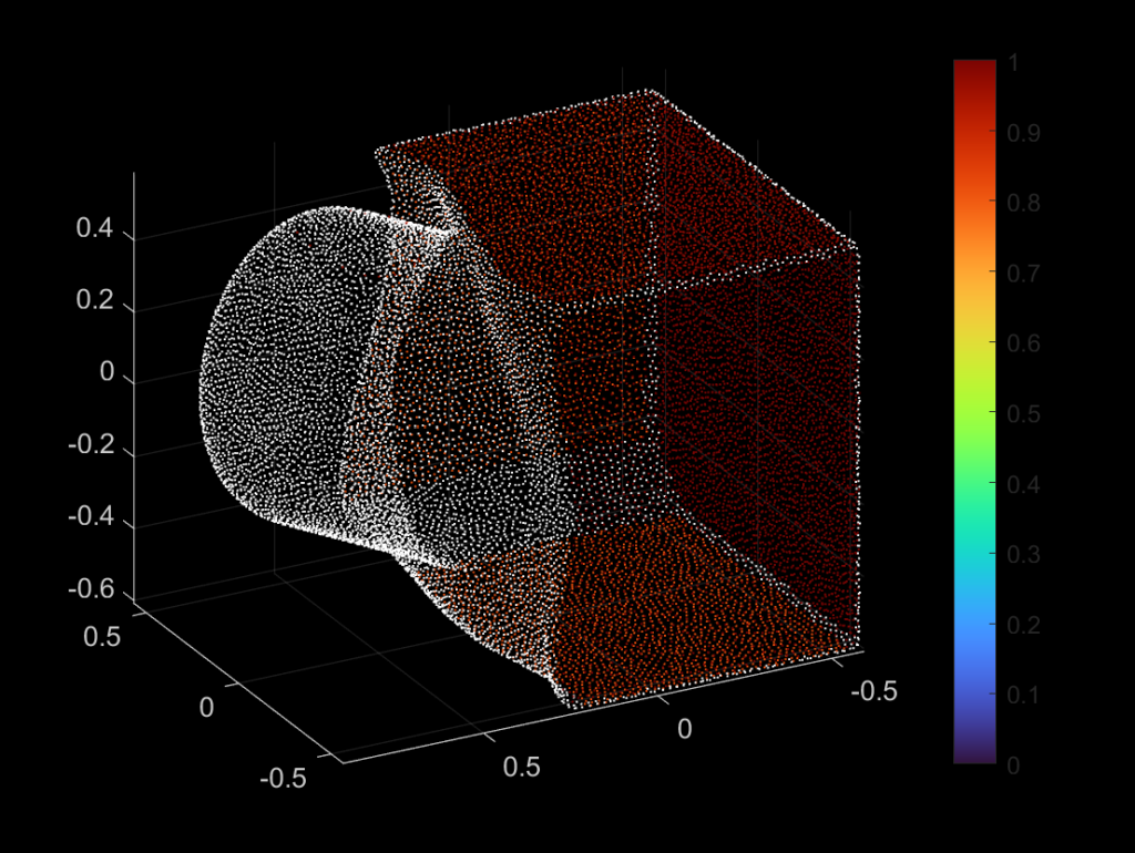
We define a plane P as the dominant plane of a 3D point cloud if the number of points defined in the 3D point cloud located on the plane P is no less than the number of points on any other plane. For example, consider the following object defined by a 3D point cloud. If we assume the number of points on a face is proportional to the area of the face, then \(P_2\) is more likely to be the dominant plane than \(P_1\) since the area of \(P_2\) is greater than that of \(P_1\). So, compared with \(P_1\), there are more points on \(P_2\), which makes \(P_2\) the potential dominant plane.
An object that is defined by a point cloud, where P2 is more likely to be the dominant plane than P1.
Problem Description
Given a 3D point cloud as the input model, we aim to detect all the planes in the model. To obtain a decent detection result, we divide the problem into two separate parts:
Part 1: Find the dominant plane \(P\) from a given 3D point cloud. This subproblem can be solved by the RANSAC Algorithm.
Part 2: Find all other planes contained in the 3D point cloud. This subproblem can be successfully addressed if we iteratively repeat the following two steps: (1). remove all the points on plane \(P\) (obtained from Part 1) from the given point cloud. (2). repeat the RANSAC algorithm with respect to the remaining points in the point cloud.
The RANSAC Algorithm
An Introduction to RANSAC
The RANSAC algorithm is a learning technique that uses random sampling of observed data to best estimate the parameters of a model. RANSAC divides data into inliers and outliers and yields estimates computed from a minimal set of inliers with the most outstanding support. Each data is used to vote for one or more models. Thus, RANSAC uses a voting scheme.
Workflow & Pseudocode
RANSAC achieves its goal by repeating the following steps:
Sample a small random subset of data points and treat them as inliers.
Take the potential inliers and compute the model parameters.
Score how many data points support the fitting. Points that fit the model well enough are known as the consensus set.
Improve the model accordingly.
This procedure repeats a fixed number of times, each time producing a model that is either rejected because of too few points in the consensus set or refined according to the corresponding consensus set size.
The pseudocode of the algorithm is recorded as below:
function dominant_plane = ransac(PC)
    n := number of points defined in point cloud PC

    max_iter := max number of iterations

    eps := threshold value to determine data points that are
           fit well by model (a 3D plane in our case)

    min_good_fit := number of nearby data points required to
                    assert that a model (a 3D plane in our
                    case) fits well to data

    iter := current iteration

    best_err := measure of how well a plane fits a set of
                points. Initialized with a large number

    % store dominant plane information
    % planes are characterized as [a,b,c,d], where
    % ax + by + cz + d = 0
    dominant_plan = zeros(1,4);

    while iter < max_iter
        maybeInliers := 3 randomly selected values from data
        maybePlane := a 3D plane fitted to maybeInliers
        alsoInliers := []
        for every point in PC not in maybeInliers
            if point_to_model_distance < eps
                add point to alsoInliers
            end if
        end for

        if number of points in alsoInliers is > min_good_fit
            % the model (3D plane) we find is accurate enough

            % this betterModel can be found by solving a least
            % square problem.
            betterPlane := a better 3D plane fits to all
                        points in maybeInliers and alsoInliers
            err := sum of distances from the points in
                   maybeInliers and alsoInliers to betterPlane
            if err < best_err
                best_err := err
                dominant_plane := betterPlane
            end if
        end if

        iter = iter + 1;
    end while
end
Detect More Planes
As mentioned before, to detect more planes, we may simply remove the points that are on the dominant plane \(P\) of the point cloud, according to what is suggested by the RANSAC algorithm. After that, we can reapply the RANSAC algorithm to the remaining points, and we get the second dominant plane, say \(P’\) of the given point cloud. We may repeat the process iteratively and detect the planes one by one until the remaining points cannot form a valid plane in 3D space.
The following code provides a more concrete description of the iterative process.
% read data from .off file
[PC, ~] = readOFF('data/off/330.off');

% A threshold eps is set to decide if a point is on a detected
% plane. If the distance from a point to a plane is less than
% this threshold, then we consider the point is on the plane.
eps = 2e-3;

while size(PC, 1) > 3
    % in the implementation of ransac, if the algorithm cannot
    % detect a plane using the existing points, then the
    % coefficient of the plane (ax + by + cz + d = 0) is a
    % zero vector.
    curr_plane_coeff = ransac(PC);

    if norm(curr_plane_coeff) == 0
        % remaining points cannot lead to a meaningful plane.
        % exit loop and stop algorithm
        break;
    end

    % At this point, one may add some code to visualize the
    % detected plane.

    % return the indices of points that are on the dominant
    % plane detected by RANSAC algorithm
    [~, idx] = pts_close_to_plane(PC, curr_plane_coeff, eps);

    % remove the points on the dominant plane.
    V(idx,:) = [];
end
Results
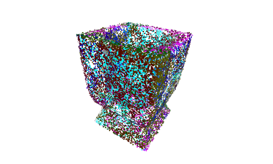
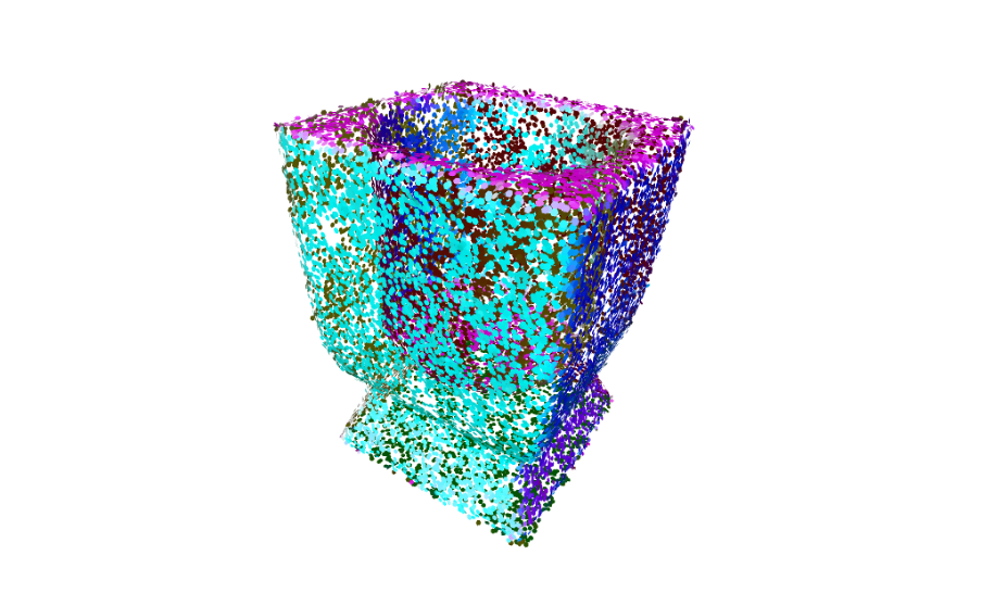
RANSAC algorithm gives good results with 3D point clouds that have planes made up of a good number of points. The full implementation is available on SGI’s Github. This method is not able to detect curves or very small planes. The data we used to generate these examples are the Mechanical objects (Category 17) from this database.
Successful Detections
Mech. Data Model Number
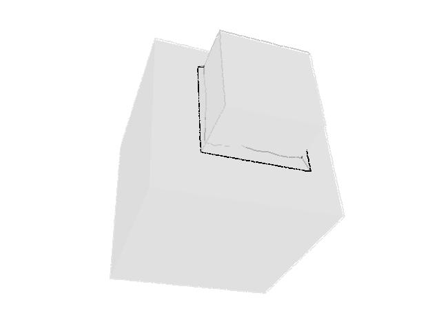
Model Object
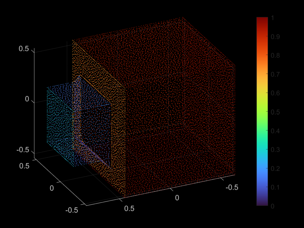
RANSAC Plane Detection Result
330
331
In the third column, red dots are points on the most dominant plane, followed by blue and green dots are points on the least dominant plane.
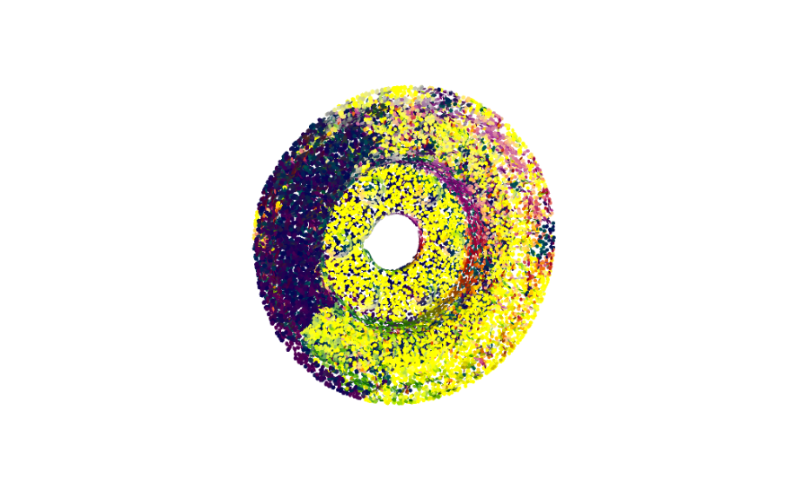
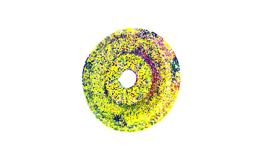
Unsuccessful Detections
Mech. Data Model Number
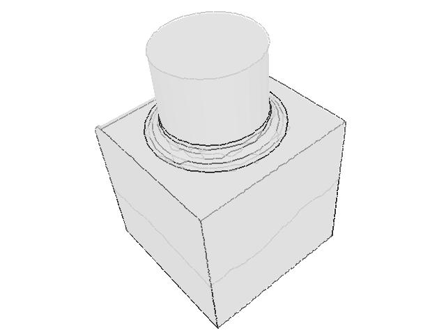
Model Object
RANSAC Plane Detection Result
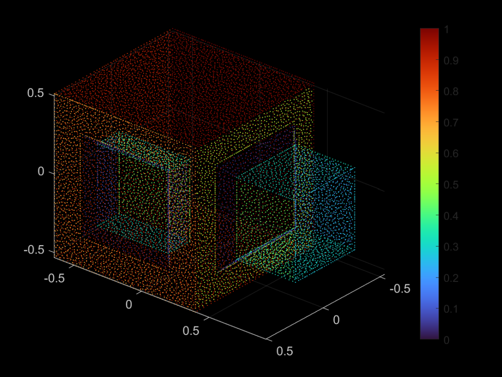
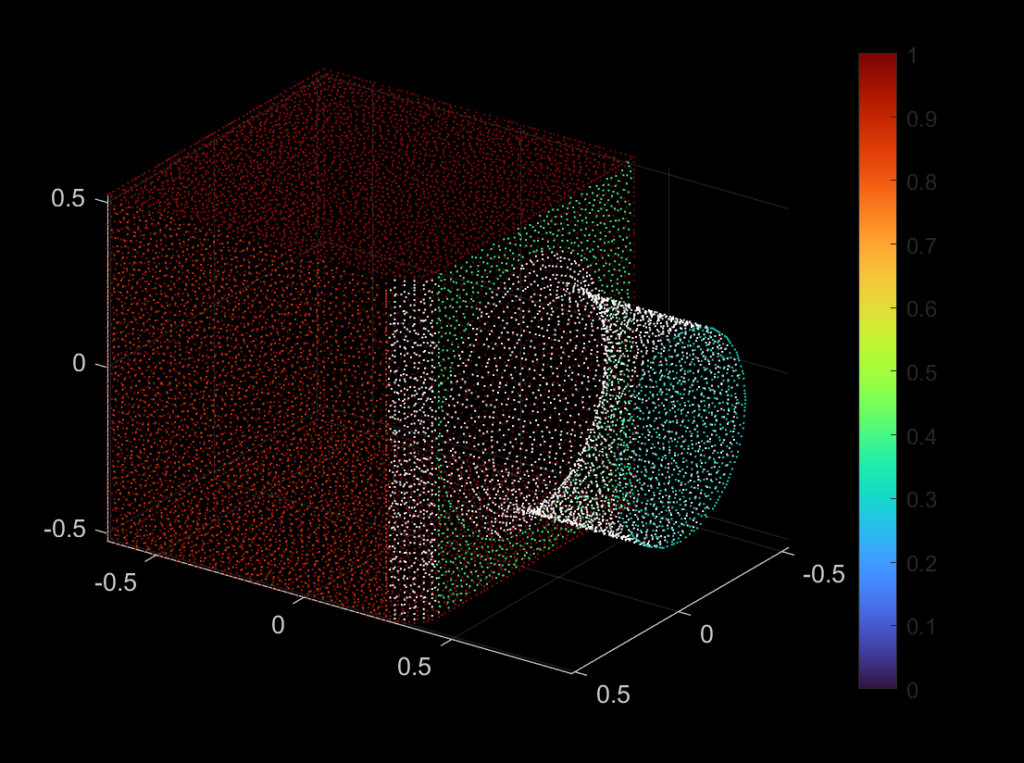
332
338
In the third column, red dots are points on the most dominant plane, followed by blue and green dots are points on the least dominant plane. White points are the ones that cannot be characterized as a plane by the RANSAC algorithm.
Limitations and Future Work
As one may observe from the successful and unsuccessful detections, the RANSAC algorithm is good at detecting planar surfaces. However, the algorithm usually fails to detect a curved surface, because we are fitting the three randomly selected points using a plane equation as our base model. If we change this model to be a curved surface, then theoretically speaking, the RANSAC algorithm should be able to detect a curved plane. We may apply a similar fix if we want to perform line detection.
Moreover, we may notice that the majority of surfaces in our test data can be represented easily by an analytical formula. However, this pre-condition is, in general, not true if we choose an arbitrary point cloud. If this is the case, the RANSAC algorithm is unlikely to output an accurate detection result, which leads to more extra work.
By Tiago Fernandes, Anna Krokhine, Daniel Scrivener, and Qi Zhang
During the first week of SGI, our group worked with Professor Misha Kazhdan on a virtually omnipresent topic in the field of geometry processing: algorithmically assigning normal orientations to point clouds.
Introduction
While point clouds are the typical output of 3D scanning equipment, triangle meshes with connectivity information are often required to perform geometry processing techniques. In order to convert a point cloud to a triangle mesh, we first need to orient the point cloud — that is, assign normals \(\{n_1, … n_n\}\) and signs \(\{\alpha_1, … \alpha_n\}\) to the initially unoriented points \(\{p_1, … p_n\}\).
To find \(n_i\), we can locally fit a surface to each point \(p_i\) using its neighborhood \(N(i)\) and use its uniquely determined normal. More difficult, however, is the process of assigning consistent signs to the normals. In order to evaluate the consistency of the signs, we have the following energy function, which we minimize over alpha:
\(E(\alpha)=\alpha^T\cdot E\cdot \alpha\)
Where \(\alpha \in \{-1, +1\}^n\) is the vector of signs and \(\tilde{E}_{ij} = \begin{cases} \frac{\langle N_i(p_i), N_i(p_j)\rangle \cdot \langle N_j(p_i), N_j(p_j) \rangle}{2} & i \sim j \\ 0 & \text{otherwise}\end{cases}\).
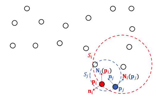
Two neighboring points, labelled pi and pj, have their normal orientations determined by the mapping of each normal onto the other point’s best-fit surface.
As shown in the diagram, \(N_i(p_j)\) is the normal assigned to \(p_j\) by the local surface fitted at \(p_i\). Greater values of \(E_{ij}\) indicate more consistent normal orientations, and thus we encourage neighboring points to have similar orientations.
Our goal is to obtain a set of signs minimizing this energy function, which is difficult to calculate on the full point set at once. To simplify the process, we looked at algorithms built on a hierarchical approach: we solve the problem first on small clusters of points, recursively building larger solutions until we’ve arrived at the initial problem.
Within this general algorithmic structure, we explored different possibilities as to the surfaces used to represent each cluster of points locally. Prof. Kazhdan had previously tried two approaches, one linear and the other quadratic. The linear approach assigns best-fit planes to the neighborhood around each point, whereas the quadratic approach uses general quadratic functions of best fit.
While these techniques provided a good foundation, we identified several failure cases upon experimenting with various point clouds. The linear approach works well on simple faces, but struggles to maintain consistent orientation around sharp features like edges. This is best demonstrated with the flower pointset, where the orientations of the normals are inverted in some clusters. The quadratic approach does better with fitting to distinctive features but overfits to what should be more simple surfaces, producing some undesirable outcomes such as the flower and vase seen below.
flower.xyz generated with linear fitting
Vase generated with quadratic fitting
Defining New Fits: First Attempt
Given that the linear and quadratic fits presented their own unique shortcomings, it became clear that we needed to experiment with different surface representations in order to find suitable fits for all clusters. Thanks to the abstract nature of our framework, there were few limitations on how the implicit surface needed to be defined; the energy function requires only a method for querying the gradient as well as a means of flipping the gradient’s sign, which leaves many options for implementation.
Our first geometric candidate was the sphere, a shape that approximates corners well due to the fact that it has curvature in all three directions. Additionally, fitting a set of points to a sphere is fairly straightforward: we used the least-squares approach described here, which, in implementation terms, is no more difficult than setting up a linear system and solving it. Unfortunately, the simplest solutions are not always the best solutions…
flower.xyz generated with spherical fitting
The spherical fitting wasn’t able to deal with sharp edges as expected, incorrectly matching the normal orientations when merging clusters close to those edges. It also generated some noise across the surface. But the process of designing the spherical fit gave us a solid idea on how to model other surfaces (and also helped to demystify some esoteric C++ conventions).
Parabolic Fit
We’ve established that since the surface may curve, a linear fit can be non-faithful to the features of the original pointset. Conversely, the generic quadratic fit has the potential to produce undesirable surface representations such as hyperbolas or ellipsoids. To this end, we introduced a parabolic fit, which improves upon the linear fit via the addition of a parameter.
By constructing a local coordinate frame where the normal from the linear fit serves as our z-axis, we were able to fit \(z=a(x^2 + y^2)\) with energy \(E_{loss} = \sum\limits_{i} (z_i – a(x_i^2+y_i^2))^2\). From this we obtained \(a = \frac{\sum_i z_i (x_i^2+y_i^2 ) }{\sum_i(x_i^2+y_i^2 )^2}\) yielding an \(a\) that minimizes this energy. By observing that \(z_i=\langle \vec{p_0 p_i} ,n \rangle, x_i^2+y_i^2=||\vec {p_0 p_i} \times n||^2\) , we derived a formula that is easier to represent programmatically: \(a = \frac{\sum_i \langle \vec{p_0 p_i} ,n \rangle ||\vec {p_0 p_i} \times n||^2 }{\sum_i||\vec {p_0 p_i} \times n||^4}\).
We calculated the gradient in a similar manner. Since locally \(\nabla ( z – a(x^2+y^2)) = (-2ax,-2ay,1) = -2a(x,y,0) + (0,0,1)\), then \(\nabla ( z – a(x^2+y^2)) = -2a\cdot \mbox{Proj}(\vec{p_0 p_i}) + \vec{n}\), where \(\mbox{Proj}( )\) projects vectors into the plane obtained in the original fit, which is written in a more code-friendly manner as \(\mbox{Proj}(\vec{x}) = \vec{x} – \langle \vec{x}, \vec{n} \rangle \vec{n}\). Finally, the gradient could be expressed as \(\nabla ( z – a(x^2+y^2)) = -2a(\vec{x} – \langle \vec{x}, \vec{n} \rangle \vec{n}) + \vec{n}\).
Our implementation of the parabolic fit generally works better than the linear fit, correcting for some key errors. It works particularly well on smooth, curved point clouds.
As for the flower dataset, however, the performance was still sub-par. When we examined some of the parabolic fits using a tool to visualize the isosurface, we found the following problem with some of the normals:
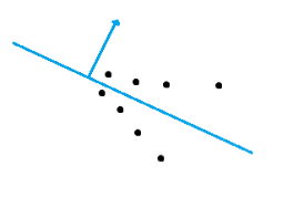
The normal of the best-fit plane doesn’t align with the best-fit parabola.
In this example, \(\vec{p_0 \bar p}\) would serve as a better normal vector than \(\vec{n}\), so we decided to implement a “choice” between the two. To avoid swapping the normal on flat point clouds (where the original normal serves its purpose quite well) we determined a threshold to handle this. Intuitively, a point cloud encoding an edge will yield a larger \(||\vec{p_0 \bar p}||\):
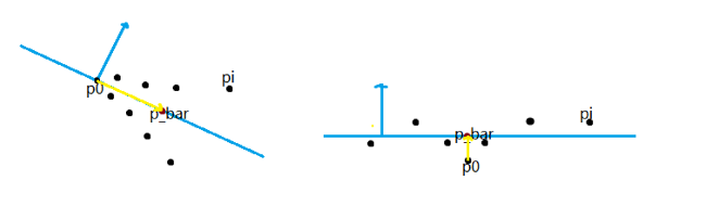
Two cases: one in which the cluster encodes an edge (left), and one in which the cluster encodes a plane (right)
To obtain a good threshold value, we used the local radius \(d_{max} = \max _{i} ||\vec{p_0 p_i}||\) and then picked a $ c$ that seems to work with our dataset (related to the size of each neighborhood), such that when \(||\vec{p_0 \bar p}|| < d_{max}/c\), we can assume the cluster is flat, whereas when \(||\vec{p_0 \bar p}||\ge d_{max}/c\) we expect it to be sharp.
Another comparison of the two cluster cases (angular versus flat local geometry). Note the relative sizes of p_bar and dmax.
In practice, this idea works well on flower.xyz when \(c \ge 12\) — the parameter is rather sensitive and can yield poor results on some point clouds if not tuned properly.
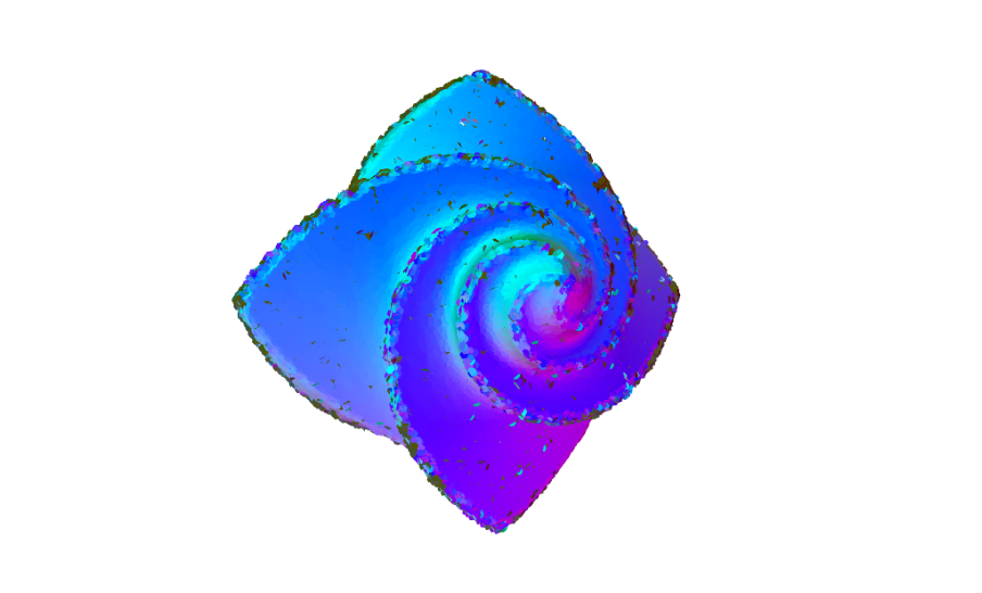
flower.xyz with parabolic fitting
Hybrid Methods: The Associative Fit
The parabolic fit provided a lot of hope as to how we could definitively address large variations in curvature. Recalling that the quadratic fit worked well for some types of clusters and that the linear fit worked well for others, the advantages of somehow being able to merge the two methods by leveraging both of their strengths had become apparent. This observation is what ultimately gave rise to the “associative” fit, which
constructs two different fits for each cluster, and
chooses the best fit by comparing the performance of the first fit to a user-specified threshold value.
The first fit’s performance is assessed according to a standard statistical measurement known as R-squared, which tells us, as a percentage, how much of the point cluster’s variation is explained by the chosen fit (or simply put, the correlation between the fit and the pointset). This was straightforward enough to implement with respect to our linear fit, which always serves as the first fit that AssociativeFit attempts to query. We can completely disable the linear fit when its R-squared value does not meet the threshold for inclusion, allowing us to switch to a better fit (quadratic, parabolic) for clusters where the observed variance is too great for a planar representation. As it turns out, clusters with high variance are likely to encode geometries with high curvature, which makes the use of a higher-degree fit appropriate.
Many of our best results were obtained using the associative fit, and we were pleased to see clear improvements over the original single-fit approaches. The inclusion of a threshold parameter does necessitate a lot of hands-on trial and error by the user — we’d eventually like to see this value determined automatically per-pointset, but the optimization problem involved in doing so is particularly challenging given that each point cloud has its own issues related to non-uniform sampling and density.
flower.xyz generated with associative (linear, quadratic) fitting
flower.xyz generated with associative (linear, quadratic) fitting
Quantitative Performance, Distance Weighting, and Other Touch-Ups
Aside from defining new implicit surfaces, we made a lot of other miscellaneous changes to the existing code base in order to improve our means of assessing each fit’s performance. We also wanted to provide the user with as much flexibility as possible when it came to manual refinement of the results.
At the beginning, when it came time to analyze our results, we relied heavily upon the disk-based visualization tool used to generate the images in this blog post. We also explored geometry processing techniques (mainly Poisson reconstruction) that make extensive use of the generated normals, assessing their performance as a proxy for the success of our method. These tools, however, provide only a qualitative means of assessment, essentially boiling down to whether a result “looks good.”
Fortunately, many of the point clouds in our dataset came with pre-assigned “true” normals that were then discarded by our method as it attempted to reconstruct them. We could easily use these normals as a point of comparison, allowing us to generate two metrics: similarity of normal lines (absolute value of the dot product, orientation-agnostic) and similarity of orientations (sign of the dot product). These statistics not only helped us with our debugging, but serve as natural candidates for any future optimization process that compares multiple passes of the algorithm.
The last main improvement to cover is the introduction of “weights” in the construction of each fit, or attenuating values that attempt to diminish the contribution of points farthest away from the mean. Despite having been implemented before we even touched the codebase, the weights were not used until we enabled them (previously, each fit received a weighting function that always returned a constant value rather than one of these distance-based weights). Improvements were modest in some cases and quite noticeable in others, as indicated by our results.
Pulley generated without distance weighting
Pulley generated with distance weighting
Conclusion
The problem of orienting point clouds is NP-hard in its simplest formulation, and a good approach for this task needs to take advantage of the geometric properties and structure of point clouds. By implementing more complex surface representations, we were able to significantly improve the results obtained across the 17 point clouds used for testing. The associative & parabolic fits in particular produced promising results: both were able to preserve the orientations of clusters across sharp edges and smooth surfaces alike.
Several obstacles remain with regard to our approach. The algorithm may perform poorly on especially dense point clouds or point clouds with non-manifold geometry. Additionally, our new surface representations are sensitive to manually-specified parameters, preventing this method from working automatically. Fortunately, the latter issue presents an opportunity for future work with optimization.
It was exciting to start off SGI working on a project with so many different applications in the field of geometry processing and beyond. The merit of this approach lies primarily with the fact that it provides an out-of-the box solution: once you compile the code, you can start experimenting with it right away (there are no neural networks to train, for example). We’re hopeful that this work will only continue to see improvements as adjustments are made to the various surface implementations (and there may be a part II on that front — stay tuned!)
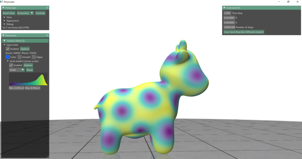
The Gray-Scott reaction-diffusion model consists of two partial differential equations: $$\frac{\partial U}{\partial t}=D_u\nabla^2U-UV^2+F(1-U)$$ $$\frac{\partial V}{\partial t}=D_v\nabla^2V+UV^2-(F+k)V.$$Using a semi-implicit approach, each \(U^{i+1}\) can be calculated as follows: \((I -{\Delta}tD_uL)U^{i+1}=U^i + {\Delta}t (F(1-U^i) – U^iV^iV^i)\). Here, \(I\) is the identity matrix, \({\Delta}t\) is change in time, \(D_u\) is the diffusion rate, \(L\) is the Laplacian of the mesh, \(F\) is the feed rate, and \(k\) is the degrading rate. Similarly, \(V^{i+1}\) can be calculated as follows: \((I -{\Delta}tD_vL)V^{i+1}=V^i + {\Delta}t (U^iV^iV^i-(F+k)V^i)\). Using Eigen‘s SimplicialLDLT solver, which uses Cholesky decomposition, we can solve for each:
Eigen::SparseMatrix<double> temp1 = (I - timeStep * du * L).eval();
Eigen::SparseMatrix<double> temp2 = (I - timeStep * dv * L).eval();

Eigen::SimplicialLDLT<Eigen::SparseMatrix<double>> solver1;
Eigen::SimplicialLDLT<Eigen::SparseMatrix<double>> solver2;

solver1.compute(temp1);
solver2.compute(temp2);

for (int i = 0; i < numSteps; i++) {
   Eigen::VectorXd UVV = U.array() * V.array() * V.array();
   Eigen::VectorXd FU = F.array() * U.array();
   U = solver1.solve((U + timeStep * (F - FU - UVV)).eval());
   Eigen::VectorXd kV = k.array() * V.array();
   Eigen::VectorXd FV = F.array() * V.array();
   V = solver2.solve((V + timeStep * (UVV - kV - FV)).eval());
}
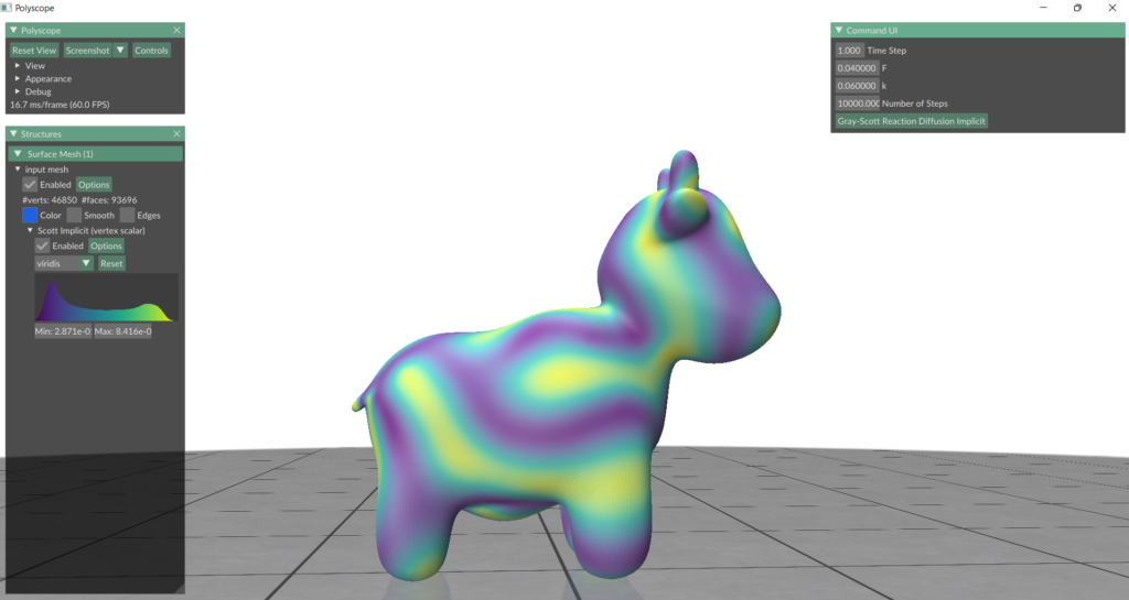
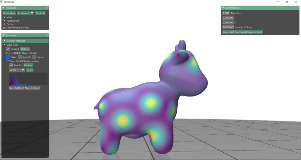
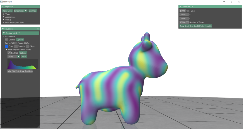
U was initialized to be 1.0 everywhere, and V was initialized to be 0.0 everywhere except in one small area where it was initialized to be 1.0. Du and Dv were set to be 1.0 and 0.5, respectively. I then modelled this onto a 3D mesh of Spot the cow using Polyscope with a time step of 1 and various F and k values, based on parameters found in Pearson’s “Complex Patterns in a Simple System” (1993). Below is a summary of the initial results. You can see various patterns formed by the Gray-Scott model.
F = 0.024 and k = 0.06 at 10,000 steps:
F = 0.04 and k = 0.06 at 10,000 steps:
F = 0.05 and k = 0.06 at 10,000 steps:
F = 0.03 and k = 0.056 at 10,000 steps:
F = 0.044 and k = 0.063 at 10,000 steps:
Acknowledgments:
Thank you to my project partners Mariem Khlifi and Gimin Nam for help with (lots of!) debugging.
Thank you to my project mentor Etienne Vouga and project TA Erick Jimenez Berumen for guidance, debugging, and resources.