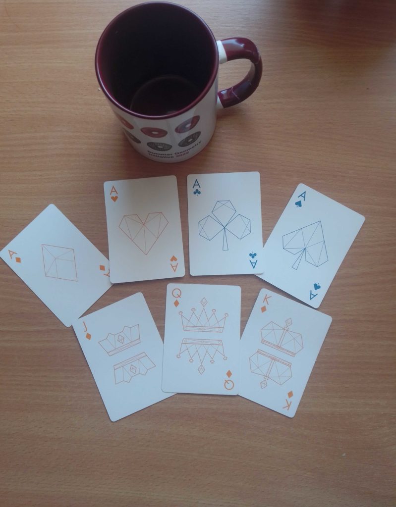
Selection of Cards from MathWorks’ Playing Cards…. and the SGI 2022 Mug.
For my first SGI blog, I have decided to combine what we have learned during the second day of the tutorial week given by the amazing Silvia Sellán to get an alternative version of the playing cards that we, fellows, have received in the swag package. The code can be found on SGI’s GitHub.
The cards are nicely designed already, so the goal is not to get a superior design but to put the knowledge we have collected into practice.
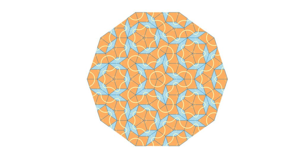
If you are curious about how the design was made by Mathworks, you can consult this website where they provide an explanation of the code that went into building the patterns. To briefly summarize the concept, the patterns were made using a Penrose Tiling, an aperiodic tiling that covers a surface with shapes such as triangles, polygons, etc. The Penrose Tiling is more distinct in larger surfaces where the tile’s repetition creates a distinct pattern.
Penrose tiling as obtained after running the steps in the Playing Cards blog.
The tiling in the deck of playing cards is much simpler than what the Penrose Tiling usually ends up looking like because the number of tiles used to divide the shapes is very small. The aim is to recreate a simple pattern using triangulation principles that we have covered during the tutorial week.
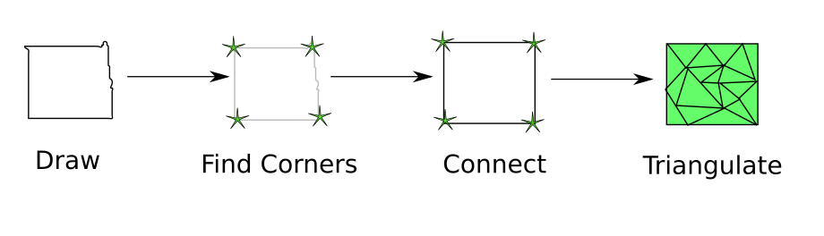
The steps making our approach, which we are going to detail in this post, can be summarized in the pipeline below:
Pipeline
The idea used to recreate the cards is based on two commands, one of them being the drawing tool from the gpltoolbox and the triangulation tool:
[V,E,cid] = get_pencil_curves(1e-6);(1)
[U,G] = triangle(V,E,[],'Flags','-q30');(2)
To recreate the style of the playing cards, we will need to transfer the drawing obtained in (1) to a polyline-based design. The drawing from get_pencil_curve is never straight, so we have to detect the existing segments and estimate their positions.
To achieve this polyline-based design, the position of the segment bounds and their connections are estimated which means that to recreate the polylines, we need to estimate the points that have corner properties and build the connections between these points.
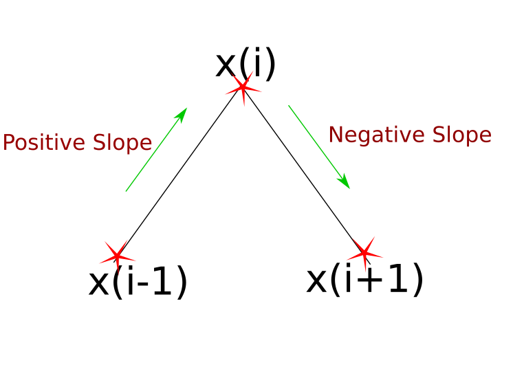
To execute the step that consists of detecting these corner points, we can use the script find_corners.m. The principle is simple: a corner point is a point \(x_{i}\) where the sign of the derivative changes when measured between \(x_{i}\)’s predecessor \(x_{i-1}\) and successor \(x_{i+1}\). The edge cases where vertical lines exist in the drawing and that yield to +/-Inf derivatives and the case of horizontal lines that have a zero derivative along the segment are also accounted for.
\(x_{i}\) is a corner with a change in the slope’s sign.
Points that satisfy this change in the slope’s sign will be considered corner candidates. At the end of the corner detection process, a pruning occurs to discard points that are very close to each other. Once we have these corner points, the polylines can be immediately seen as the connection between two consecutive corners.
Curvatures also naturally trigger this change in the slope’s sign. We do however need to distinguish between an intentional curvature and a non-intentional one caused by drawings which inherently have lines with varying degrees of curvature attributed to hand made drawings with the get_pencil_curve tool. This is solved by fixing a derivative threshold that discards very small variations.
When the polyline-based design is ready, we can run the triangulation tool as in (2) to obtain our resulting shapes.
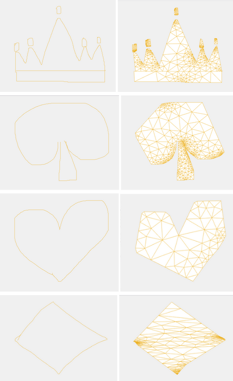
In the pictures below, we have collected the results from our algorithm which generated triangulated polyline versions of shapes created by users. The results are not perfect due to many irregularities in the original drawing. These irregularities stem from the low quality of the drawings when using a mouse instead of an actual pen.
A queen, a spade, a heart and a diamond before and after triangulation.
Some interesting observations can be made from the results of the heart and spade shapes: the algorithm converts their curved lines into two straight lines which meet at a point that showcases corner properties which validates that strong curvatures are properly considered and the inevitable ones are discarded.
And with that, we can finally say that we have our own “artsy” playing cards design or maybe this could already be Mathworks’ design in a parallel universe!
By SGI fellows Alejandro Pereira and Vivien van Veldhuizen
On the last day of the tutorial week, Nicholas Sharp gave a talk about robustness and debugging in geometry processing. He explained that there are a lot of interesting software tools available for geometry processing, but it is sometimes hard to make these tools robust to different types of data. This is especially true in geometry processing, where there are a lot of different complex data structures such as meshes. Software tools not being robust to different sorts of data, leads to a lot of the available tools becoming unusable, or results coming out wrong. It is therefore important for anyone working with geometry processing, to know what kinds of robustness problems you might encounter and how these may be solved.
Five Common Problems
Nicholas mentioned five of these common problems. The first concerned floating point numbers not being as precise as real mathematical numbers. This could lead to inaccurate data representations, which only pile up as we start computing with the less precise floating point numbers. A second problem to think about was different types of solvers. Nicholas mentioned that we often use numerical solvers in geometry processing, but that some types are a lot more fast and reliable (such as dense linear solvers) than others (for example quadratic or nonlinear solvers). Another common problem Nicholas mentioned was the problem of “bad” meshes. Preloaded meshes could for example have orientation problems, contain overlapping vertices or be nonmanifold. Moreover, even if the meshes were all structured correctly, if we want to run simulations on these meshes, a given algorithm might work on one mesh but not the other. This is because in visual computing, algorithms and inputs (in this case our meshes) are not designed together. Instead, algorithms are just a part of a pipeline and are expected to work on any input data, which is of course not always feasible in practice. Finally, Nicholas briefly talked about machine learning for geometry processing, which is often marketed as an alternative to classic geometry processing. He mentioned that actually, machine learning methods often still contain a lot of geometry processing operations under the hood, so we might still run into any of the problems mentioned above, which might also impact our machine learning results.
To show us what some these problems might look like in practice, Nick gave us two Matlab “puzzles” that we had to solve. Each of these Matlab exercises had some sort of robustness problem and our goal was to find out what these problems were and solve them.
Puzzle 1
In the first exercise, we want to plot a simple mesh. Nothing too complicated right? Once we have a matrix of vertices V and a matrix for the faces F, it’s just a simple case of running:
>> tsurf(F, V)
However, we get an error:
Error using patch
Value must be of numeric type and greater than 1.

Error in trisurf (line 95)
h = patch('faces',trids,'vertices',[x(:) y(:) z(:)],'facevertexcdata',c(:),...

Error in tsurf (line 132)
t_copy = trisurf(F,V(:,1),V(:,2),V(:,3));
So, what happened? MATLAB told us the error comes from the patch function, so we call patch directly to see what is happening:
>> patches('Faces', F, 'Vertices', V)
Error using patch
Value must be of numeric type and greater than 1.
Because patch only uses V and F, the problem must be in either one of those variables. What if we explicitly give it the X, Y, and Z coordinates of the vertices to plot?
Yes, progress! We plotted something, and we can see that it is a duck. The vertices matrix seems to be correct, so perhaps i is the faces F that is the problem
Remember the error in the patch function? “Value must be greater than 1.” Well, if you come from a different coding background such as Python, you know that arrays start at index=0. However, this is not the case in MATLAB, where indices start at 1. This means we just need to add 1 to F to fix the problem.
>> F= F+1
>> tsurf(F,V)
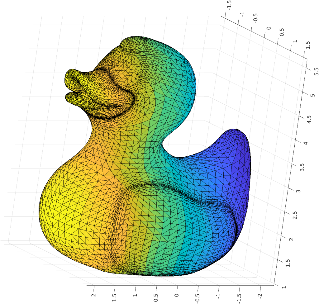
The correctly loaded mesh of a duck
Success! We have a lovely duck. Alternatively, we could have used tsurf(F+1,V) and it would also work.
Sometimes error and warnings may be a little intimidating, but if we go step by step from the first error we can find that the source is something as simple as changing a 0 to a 1.
Puzzle 2
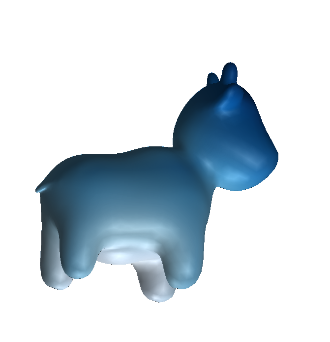
For the next exercise, our objective was to compute the geodesic distances along the surface of a ‘meshified’ cow.
For that we will use the 'heat_geodesic' function. In this case, running the function results in the following error:
>> dists = heat_geodesic(V,F,1);
Warning: Matrix is singular, close to singular or badly scaled.
Results may be inaccurate. RCOND = NaN.
> In min_quad_with_fixed/solve (line 409)
In min_quad_with_fixed (line 103)
In heat_geodesic (line 199)
Here the problem is a little more complicated: in our quadratic solver, one of the matrices is singular. This means, among several other equivalent propositions, that the determinant of said matrix is 0.
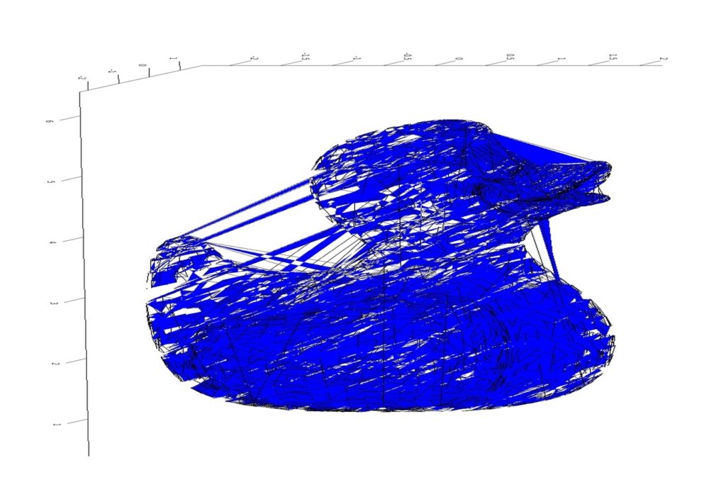
For now, let’s try to visualize what the mesh looks like using tsurf(F,V):
Something is wrong with this mesh…
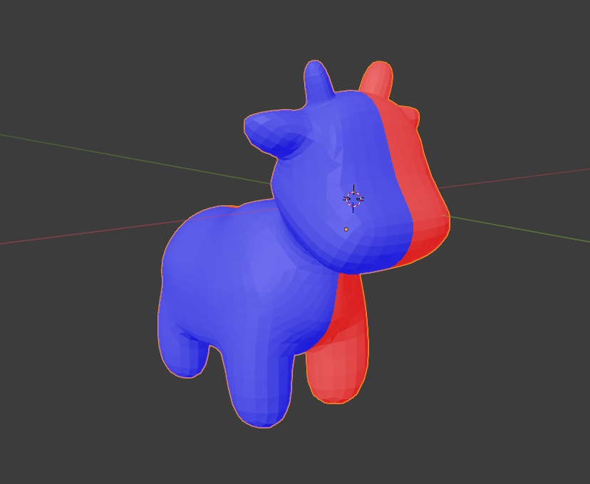
At first glance, there seems to be nothing wrong. The trick is to realize that some of the vertices in the above mesh are too close to each other. This results in the matrix becoming singular. One way to solve this is to merge vertices that are closer to a certain threshold. In this case, a threshold of 0.0001 m is enough to remove 120 vertices. The result:
Correct rendering of Spot the cow
Finally, we get the desired result!
In conclusion: debugging is not only important but also fun! Spending time trying to understand the problem, creating our own hypothesis of what the output should be, and then testing them is what science is all about.
Many of the SGI fellows experienced an error using the png2poly function from the gptoolbox: when applied to the example picture, the function throws an indexing error and in some cases makes Matlab crash. So, I decided to investigate the code.
The function png2poly transforms a png image into closed polylines (polygons) and applies a Laplacian smoothing operation. I found out that this operation was returning degenerated polygons, which later in the code was crashing Matlab.
But first, how does Laplacian smoothing work?
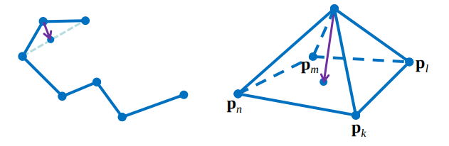
I had never seen how a smoothing operation works, and I was surprised with how simple the idea of Laplacian smoothing is. It’s an iterative operation, and at each iteration the positions of the vertices are updated using local information, the position of neighbor vertices.
New position of vertices after one iteration (credit: Stanford CS 468).
In polylines, every vertex has 2 neighbors, apart from boundary vertices, to which the operation is not applied. For closed polylines, Laplacian smoothing converges to a single point after many iterations.
The Laplacian matrix \(L\) can be used to apply the smoothing for the whole polyline at once, and a Lambda parameter (0 ≤ λ ≤ 1) can be introduced to control how much the vertices are going to move in one iteration:
\[p \gets p + \lambda L p\]
The best thing about Laplacian smoothing is that the same idea pleasantly applies for meshes in 3D! The difference is that in meshes every vertex has a variable number of neighbors, but the same formula using the Laplacian matrix can be used to implement it.
For more details on smoothing, check out this slide from Stanford, from which the images in this post were taken. It also talks about ways to improve this technique using an average of the neighbors weighted by curvature.
What about the bug?
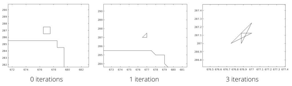
The bug was the following: For some reason, the function that converts the png into polygons was generating duplicate vertices. Later in the code, a triangulate function is used on these polygons, and the duplicate vertices by themselves make the function crash. But even worse, when smoothing is applied to a polygon with duplicate vertices, strange things happen. Here’s an example of a square with 5 vertices (1 duplicated); after 3 iterations it becomes a non-simple polygon:
You can try to simulate the algorithm to see that it happens.
Also, the lambda parameter used was 1.0, which was too high, making small polygons collapse or generating new duplicate points, so I proposed 0.5 as the new parameter. For closed curves, Laplacian smoothing will converge to a single point, making the polygon really small after many iterations, which is also a problem for the triangulation function. In most settings, these converged polygons can be erased.
Some other problems were also found, but less relevant to be discussed here. A pull request was merged into the gptoolbox repository removing duplicate points and fixing the other bugs, and now the example used in the tutorial week should work just fine. The changes I made don’t guarantee that the smoothing operation is not generating self-intersection anymore, but for most cases it does.
Fun fact: There’s a technique for finding if a polygon has self-intersection called sweep line, which works in \(O(n\log n)\)—more efficient than checking every pair of edges!
The things I learned
Laplacian smoothing is awesome.
It’s really hard to build software for geometry processing that works properly for all kinds of input. You need to have complete control over degenerate cases, corner cases, precision errors, … the list goes on. It gets even harder when you want to implement something that depends on other implementations, that may by themselves break with certain inputs. Now I recognize even more the effort of professor Alec Jacobson and collaborators for creating gptoolbox and making it accessible.
Big thanks to Lucas Valença, for encouraging me to try and solve the bug, and to Dimitry Kachkovski, for testing my code.
By SGI Fellows Xinwen Ding and Miles Silberling-Cook
The authors of this article appreciate Derek Liu and Eris Zhang for their awesome lectures on the third day of SGI. The rest of this summary is based on what we learned from their lectures.
Introduction
One of the motivations for shape deformation is the desire of reproducing the motion of a given initial shape as time evolves. It is clear that modeling every piece of information associated with the initial shape can be hard and unnecessary. So, a simple but nice-looking deformation strategy is needed. During the lecture, SGI fellows were introduced two deformation strategies listed below.
Energy-based Deformation: This method turns the deformation problem into an optimization problem, where possible objective functions can be Dirichlet Energy (\(E = \int_{M} ||\nabla f||^2 dx\)), Laplacian Energy (\(E = \int_{M} ||\Delta f||^2 dx\)), or Conformal Energy. It is worth mentioning that the nonlinear optimization problems are, in general, difficult to solve.
Direct Method: We mainly refer to a method called Linear Blend Skinning (LBS). In this method, we predefine a sequence of movable handles. Furthermore, we assume the movement of every handle will contribute linearly to the final coordinate of our input vertex. Based on this assumption, we write down the equation for calculating the target position: \(u_i = \displaystyle\sum_{j = 1}^{\text{# of handles}} w_{ij} T_j v_i\), where \(v_i, u_i\) are the \(i^{th}\) input and output vertices, respectively, \(w_{ij}\) is the weight, and \(T_j\) is the tranformation matrix of the \(j^{th}\) handle recording rotation and transformation in terms of homogeneous coordinates.
The remaining part of this summary will focus on the Linear Blend Skinning (LBS) method.
Workflow
The process of a 2D LBS deformation can be divided into three steps:
Step 1: Define the handles.
Step 2: Compute the weights \(w_{ij}\) and store the tranformation matrix \(T_j = \begin{bmatrix}\cos\theta & -\sin\theta & \Delta x \\ \sin\theta & \cos\theta & \Delta y\end{bmatrix}\), where the first two columns of \(T_j\) denote the rotation of the \(j^{th}\) handle, and the last column denotes the shift. Notice that in this case the \(i^{th}\) vertex should be \(v_i = \begin{bmatrix} v_x \\ v_y \\ 1\end{bmatrix}\).
Step 3: Put all parts together and compute \(u_i = \displaystyle\sum_{j = 1}^{\text{# of handles}} w_{ij} T_j v_i\).
A concrete example will be given in the final section.
Weight Calculation
Requirements on weights:
To minimize the artifacts in our deformation, we need to be smart when we generate the weights. Briefly speaking, we want our weights to satisfy the following criteria:
Smooth: the weight function should be \(C^{1}\) differentiable. This can be achieved by introducting the Laplacian operator.
Local: the effective area in a 2D domain should be within some neighborhood of the handle.
Shape aware: the effective area in a 2D domain should not cross the boundary of our domain of interest.
Sum up to 1.
Let \(\Omega\) be the domain of the interest, and \(w\) be the weight. Based on the aforementioned requirements, we can use the following minimization problem to characterize the weights.
\begin{equation}
\begin{aligned}
&\min_{w} \int_{\Omega} || \Delta w||^2 dx \\
&\textrm{s.t.} w(j^{th} \text{handle}) = e_j \hspace{20pt} \text{($e_j$ is a standard basis vector)}
\end{aligned}
\end{equation}
Discretize the Laplacian Operator
One may notice that in the objective function of the above optimization problem, we introduced a Laplacian operator. Luckily, we can play some math tricks to discretize the Laplacian operator, namely \(\Delta = M^{-1}C\), where \(M\) is the diagonal mass matrix, and \(C\) is the cotangent formula for the Laplacian.
With this knowledge in mind and with some knowledge from Finite Element Method, we can rewrite the objective function into a quadratic form.
\[
\int_{\Omega} || \Delta w||^2 dx
= ||M^{-1}Cw||_{M}^2
= (M^{-1} C w)^{T} M (M^{-1} C w)
= w^{T} C^{T} M^{-1} C w
\]
Let \(B = C^{T} M^{-1} C\), then we have \(\int_{\Omega} || \Delta w||^2 dx = w^{T} C^{T} M^{-1} C w = w^{T} B w\). Moreoever, we name the matrix \(B\) as bilaplacian or square Laplacian. Hence, the optimization problem is rewritten as follows:
\begin{equation}
\begin{aligned}
&\min_{w} w^{T} B w \\
&\textrm{s.t.} w(j^{th} \text{handle}) = e_j \hspace{20pt} \text{($e_j$ is a standard basis vector)}
\end{aligned}
\end{equation}
Solution Derivation to the Optimization Problem
Recall that \(w_{ij}\) is the degree to which vertex \(i\) is effected the motion of handle \(j\). To form our constraint, we pick a vertex for each handle that will only be affected by that handle. This constraint is much easier to express when the fixed weightings are separated from the free weightings, so we re-organize the weightings as \(w = [x, y]\). In this notation, \(x\) contains the free variables for the non-handle vertices, and \(y\) contains the fixed weighting for each handle. The boundary can now be concisely stated as \(y = \mathbb{I}\).
We now solve for the \(x\) that minimizes \([x \mid y]^T B [x \mid y]\). Following Derek Liu and Eris Zhang’s lead, we use subscripts to express the indices of \(B\) pertaining to either \(x\) or \(y\).
As expected, this yields another quadratic equation. Differentiating gives:
\begin{equation}
\frac{\partial E}{\partial x}
= 2 A_{x,x,} x + \left(B_{x,y} + B_{y,x}^T \right) y
\end{equation}
and the extremizer is therefore \(x = \left( -2A\right)^{-1}\left(B_{x,y} + B_{y,x}^T \right) y\).
Code Implementation and Acceleration
Implementation
To calculate the solution in Matlab, see the following.
function W = compute_skinning_weight(V,F,b)
% V: Vertices
% F: Triangles
% b: Handle vertex indices

% Compute the Laplacian using the cotangent-matrix.
L = -cotmatrix(V,F);

% Compute the mass matrix.
M = massmatrix(V,F);

% Compute the BiLaplacian
B = L*(M\L);

% Create a list of non-handle verticies
a = setdiff(1:size(V,1), b);

% Initialize the fixed handle constraint
y = eye(length(b));

% Compute the minimum
A = Q(a,a);
B = (Q(a,b) + Q(b,a).') * y;
x = (-2*A) \ B;

% Assemble the final weight matrix
W(a,:) = x;
W(b,:) = y;
end
Once the weightings are done, we can propagate the transformation of the handles to the mesh (using homogeneous coordinates) as follows:
function [U] = linear_blend_skinning(V, T, W)
% V: Vertices
% T: Handle transforms
% W: Weighting matrix

U = zeros(size(V));

for i=1:size(V)

for j=1:size(T,3)
U(i,:) = U(i,:) + ( W(i,j) * [V(i,:) 1] * T(:,:,j).' );
end

end

end
Acceleration
Although the solution above guarantees correctness, this is a fairly inefficient implementation. Some of this computation can be done offline, and the nested loops are not required. The blending weights and the vertex positions can be compiled into a single matrix ahead of time, like so:
function C = compile_blending_weights(V, N, W)
% V: Vertices
% N: Number of handles
% W: Weighting matrix

for i=1:length(V)
v = repmat( [V(i,:), 1], 1, N)';
wi = reshape(repmat(W(i, :), 3, 1), [], 1);
C(:,i) = v.*wi;
end
end
Then propagating the transform is as simple as composing it with the precomputed weightings.
function [U] = linear_blend_skinning(T, C)
% T: Handle transforms
% C: Compiled blending weights

B = reshape(T,[], size(T, 3)*size(T, 2));
U = (B*C)';
end
Shout-out to SGI Fellow Dimitry Kachkovski for providing this extra-efficient implementation!
Example: 2D Gingerbread Man Deformation
In this example, we try to implement the whole method over a gingerbread man domain. Following the define handle – computing weights – combine and transform workflow, we provide a series of video examples.
Step 1: Define handles
By click randonly on the mesh, the handles are defined according to the position of mouse.
Step 2: Computing Weights
The area where the weight function is effective is in some color other than blue.