by Jayati Sood, Uriel Martínez, Miles Silberling-Cook and Josue Perez
Introduction
The geodesic distance between two points x and y on a mesh is the length of the shortest path from x to y, along the surface. In the first and final weeks of SGI, under the mentorship of Professor Justin Solomon and Professor Nester Guillen, we worked on finding numerical approximations of geodesic distance functions that are low in accuracy and hence faster to compute.
Given a point a set \(S\) of points on the surface \(\mathcal{M}\), we can define a function \(f_S(x):\mathcal{M}\mapsto\mathbb{R}^+\) such that
\[f_S(x) = d(x, S) = \min_{y\in S} d(x,y),\]
where \(d\) is the geodesic distance function in \(\mathcal{M}\). \(f\) satisfies the eikonal equation, i.e.,
\[||\nabla f(x)||_2=1.\]
Solving the eikonal equation with \(f_{S}(x_0)=0\) gives us the geodesic distance function from a given set of points on the mesh/manifold to all other points on the mesh. However, the eikonal equation is a non-linear PDE and hard to solve. To speed up the process, we employ Perron’s method to solve for \(f_{S}(x)\) by finding the maximum of the subsolutions of the above boundary value problem, which leads to the following convex optimization problem:
Our first task was to reformulate this optimization problem for triangle meshes. By restricting paths to the edges of the mesh we arrive at the following. Take our triangle mesh to be an edge-weighted, undirected graph \(G\).
If \(S\subset G\) is the set of vertices to which we are calculating a geodesic, then the distance function \(x\mapsto d(x, S)\) is the unique solution of the following second-order cone program (SOCP):
\[ \begin{align*} \max_f& \;\; \sum \limits_{i=1}^N f(x_i) \\ \text{subject to } & \;\; f(x_i) = 0\;\forall\;x_i\in S \\ & \;\;f(x_i)-f(x_j) \leq \ell_{e} \text{ anytime } e := (x_i,x_j) \in E \end{align*} \]
We can observe from the formulation of the problem that we have two types of constraints. The number of equations we have of the first kind depends directly on the cardinality of \(S\), meanwhile, the number of equations we have of the second type depend on the cardinality of the edges on the mesh. Hence an upper bound on the number of constraints of this particular problem is \(|S|+|E|=\frac{|S|(|S|+1)}{2}\). In other words, the number of constraints in our problem grows quadratically on the amount of vertices on the mesh. Furthermore, there is no good reason why \(f\) should be linear in general, which makes solving this problem even more computationally taxing.
We found that this formulation of the problem (with paths restricted to edges) resulted in poor-quality geodesics with negligible increase in speed. For the remainder of this project we used a form closer to the original, and approximated the gradient with finite differences. Our observations about the number of constraints still apply.
Approach
The approach we took on this project to solve these inconveniences proceeds twofold.
On a first instance, we represent \(f\) in terms of a convenient linear basis, just only for building an approximate notion of distance which takes into account only the elements on the basis that influence the most the values of \(f\), in other words, we build a low resolution geodesic. For selecting this linear base we start calculating the laplacian of the mesh. Then, we select a fixed number of eigenvectors of the matrix, giving preference to those with a lower eigenvalue.
On a second instance, we require the solution of our problem to be of low resolution. We do this by imposing new linear constraints. This could be thought to be contradictory with the goal of the project, however, with the proper use of some standard tools of convex optimization, for example the active set method, in theory we could actually reduce the number of constraints in the original problem. A consequence that we observed by using this approach on reasonably behaved meshes is that the number of active constraints on the problem depends on the size of sampled basis, yielding a method that is almost independent of the cardinallity of \(S\).
Throughout the project, we used cvx in MATLAB to solve our convex program for different sets \(S\) of vertices on the mesh, concluding with \(S\) being the set of all vertices on the mesh, which gave us the distance function for all pairs of vertices. Over the course of the project, we employed various techniques to increase the efficiency of our solver, and were successful in obtaining an all-pairs geodesic distance function on the Spot mesh.
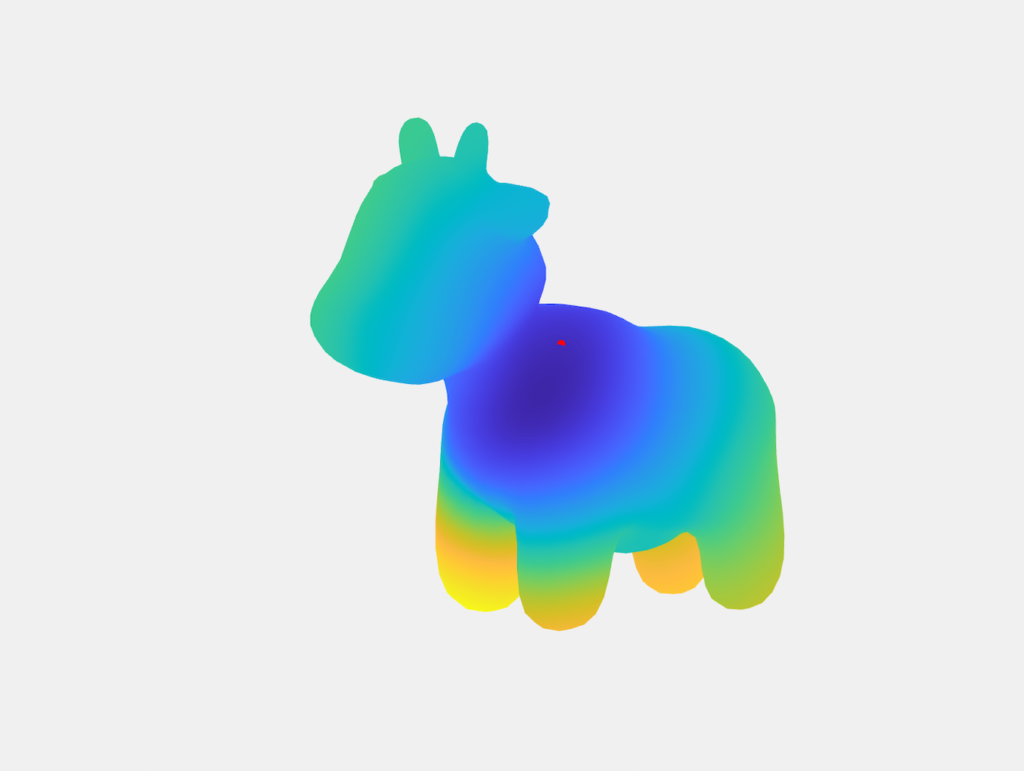
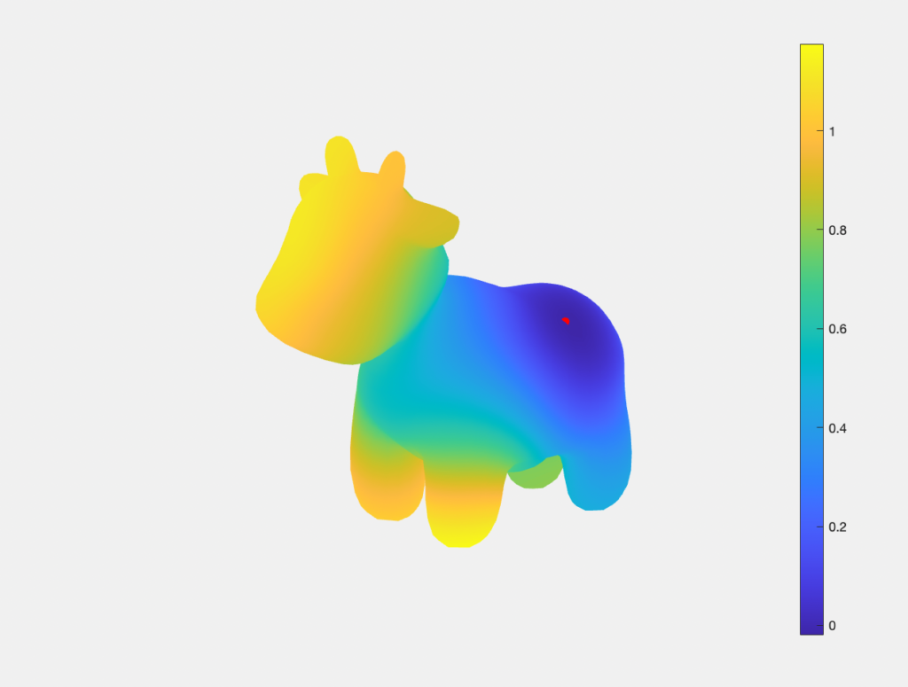
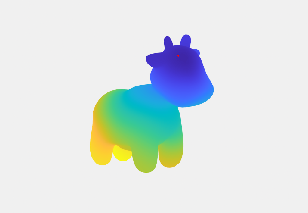
Geodesic distance function heat map
This heat map is a plot of the approximate all-pairs geodesic function for a vertex randomly sampled from Spot. The colour values represent the estimated geodesic distance from the sample vertex (red).
All-pairs geodesic distance function on Spot
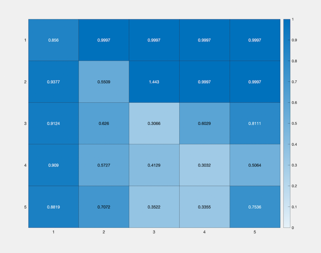
Error map
This heat map represents the change in accuracy of our approximate all-pairs geodesic distance function, with change in the number of basis vectors (vertical), and number of faces sampled (horizontal) from the Spot mesh. The colour values represent the mean relative error between the approximated function and the ground truth geodesic function, with the lightest and darkest blues being assigned to the error values “0” and “1.5”, normalized according to the observed distribution of the error values obtained. Starting with 5 faces and 5 basis vectors, and taking intervals of 5 for both, we observe that the highest accuracy is obtained along the diagonal, i.e, when the number of faces sampled equals the number of basis vectors.
During the third and fourth week of SGI, Xinwen Ding, Ahmed A. A. Elhag and Miles Silberling-Cook (week 3 only) worked under the guidance of Benjamin Jones and Prof. Adriana Schulz to explore methods that can define a continuous relaxation of CAD geometry.
Background
In general, there are two ways to represent shapes: explicit representations and implicit representations. Explicit representations are easier to model and allow local differentiable parameterizations. CAD geometry, stored in an explicit form called parametric boundary representations (B-reps), is one example, while triangle mesh is another typical example.
However, just as each triangle facet in a triangle mesh has its independent parameterization, it is hard to represent a surface using one single function under an explicit representation. We call this property discrete at the global scale. This discreteness forces us to catch continuous changes using discontinuous shape parameterization and results in weirdness and artifacts. For example, explicit representations can be incompatible with some gradient-based methods and some neural network techniques on a non-local scale.
One possible fix to this issue is to use implicit shape representations, such as signed distance field (SDF). SDFs are global functions that are continuously differentiable almost everywhere in the domain, which addresses the issues caused by explicit representations. Motivated by this, we want to play the same trick by defining a continuous relaxation of CAD geometry.
Problem Description
To define this continuous relaxation of CAD geometry, we need to find a continuous relaxation of the boundary element type. Consider a simple case where the CAD data define a geometry that only contains two types; lines and circles. While it is natural that we map lines to 0 and circles to 1, there is no type defined in the CAD geometry as the pre-image of (0,1). So, we want to define these intermediate states between lines and circles.
The task contains two parts. First, we need to learn the SDF and thus obtain the implicit shape representation of the CAD geometry. As an alignment to the input data type, we want to convert the type-blended geometry to CAD data. So next, we want to convert the SDF back to valid boundary representation by recovering the parameters of the elements we encoded in the SDF and then blending their element type.
The Method
To make it easier for the reconstruction task, we decided to learn multiple SDFs, one for each type of geometry. According to these learned SDFs, we can step into the process of recovering the geometries based on their types. Now, let us consider a concrete example. If we have a CAD shape that consists of two types of geometries, say lines and circles, we need to learn two SDFs: one for edges (part of circles) and another for arcs (part of circles). With these learned SDFs, We hope to recover all the lines that appear in the input shape from the line SDF, and a similar expectation applies to the circle SDF.
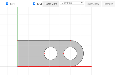
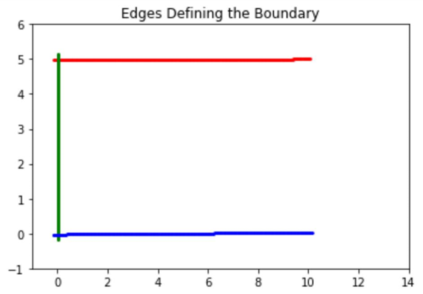
Before jumping into detailed implementations, we want to acknowledge Miles Silberling-Cook for bringing up the multi-SDF idea. Due to the time limitation at SGI, we only tested this method for edges in 2D. We start with the CAD data defining a shape in Figure 1. All the results we show later are based on this geometry.
Figure 1: Input geometry defined by CAD data.
Learned SDF
Our goal is to learn a function that maps a coordinate of a query point \((x,y) \in \mathbb{R^2}\) to a signed distance in \(\mathbb{R}\) from \((x,y)\) to the surface. The output of this function is positive if \((x,y)\) is outside the surface, negative if \((x,y)\) is enclosed by the suface, and zero if \((x,y)\) lies on the surface. Thus, our neural network is defined as \(f: \mathbb{R} ^2 \to \mathbb{R}\). For Figure 1, we learned two neural networks, the first network maps \((x,y)\) to its distance from the line edge, and the second network maps this point to its distance for the circle edge. For this task, we use a Decoder network (multi-layer perceptron, MLP), and optimize it using a gradient descent until convergence. Our dataset was created from a grid with appropriate dimensions, as these are our 2D points. Then, for each point in the grid, we calculate its distance from the line edge and the circle edge.
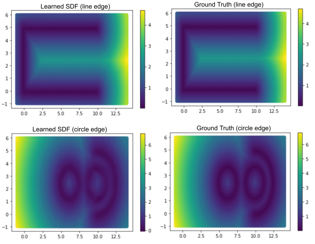
We compare the image from the learned SDF and the ground truth in Figure 2. It clearly shows that we can overfit and learn both the two networks for line and circle edges.
Figure 2: The network learned the SDF with respect to the edges (first row) and arcs (second row) of the input geometry displayed in Figure 1. We compare the learned result (left column) with the ground truth (right column).
Reconstruction
After obtaining the learned line SDF model, we need to analytically recover the edges and arcs. To define an edge, we need nothing but a starting point, a direction, and a length. So, we begin the recovery by randomly seeding thousands of points and assigning each point a random direction. Furthermore, we can only accept those points with their associated values in SDF to be close to zero (see Figure 3), which enhances the success rate of finding an edge as a part of the shape boundary.
Figure 3: we iteratively generate points until 6000 of them are accepted (i.e. SDF value small enough). The accepted points are plotted in red.
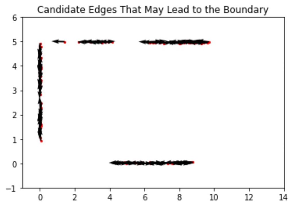
Then, we need to tell which lines are more likely to be the ones that define the boundary of our CAD shape and reject the ones that are unlikely to be on the boundary. To guarantee a fair selection, we need to fix the length of the randomly generated edges and pick the ones whose line integral of the learned line SDF is small enough. Moreover, to save more time, we approximate the integral by a finite sum, where we sum up the SDF value assumed by a fixed number of sample points along every edge. Stopping here, we have a pool of edge boundary candidates. We visualize them in terms of their starting points and direction using a quiver plot in Figure 4.
Figure 4: Starting points (red dots) and proper directions (black arrows) that define potential edges.
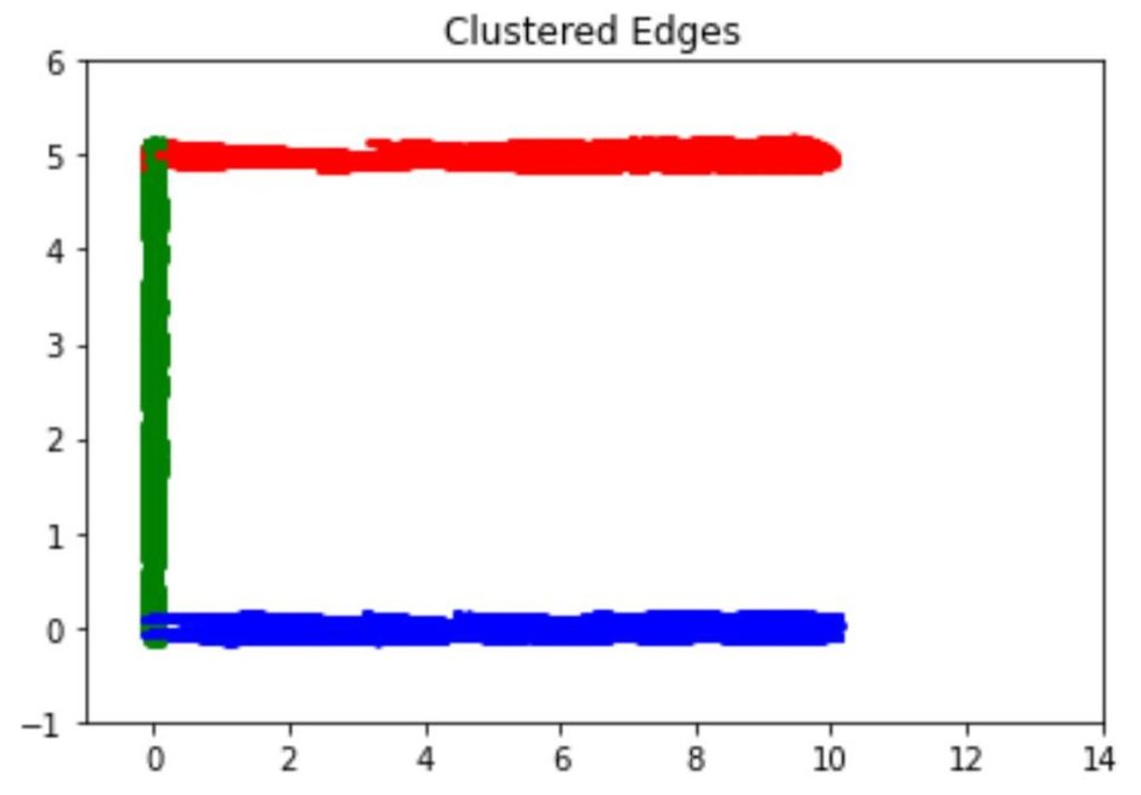
In the next step, we want to extend the candidate edges as long as possible, as our goal is to reconstruct the whole boundary. The extension ends once the SDF value of some extended point exceeds some threshold. After the extension, we cluster the extended edges using the mean shift algorithm. We adopt this clustering algorithm since it does not need to pre-determine the number of clusters. As shown in Figure 5, the algorithm successfully predicts the correct number of edge clusters after carefully tuning the parameters.
Figure 5: Clustered edges. Each color represents one cluster. After carefully tuning parameters, the optimal number of clusters found by the mean shift algorithm reflects the actual number of edges in the geometry.
Finally, we want to extract the lines that best define the shape boundary. As we set a threshold in the extension process, we simply need to choose the longest edge from each cluster and name it a boundary edge. The three boundary edges in our example, one in each color, appear in Figure 6.
Figure 6: The longest edges, one from each cluster, with parameters known.
Results
To sum up, during the project’s two-week active period, we managed to complete the following items:
We set up a neural network to learn multiple SDFs. The model learns the SDF for edge and arc components on the boundary of a 2D input shape.
We developed and implemented a sequence of procedures to reconstruct the lines from the trained line SDF model.
Future Work
Even though we showed the results we achieved during the two weeks, there are more things to improve in the future. First of all, we need to reconstruct the arcs in 2D and ensure the whole procedure to be successful in more complicated 2D geometries. Second, we would like to generalize the whole process to 3D. More importantly, we are interested in establishing a way to smoothly and continuously characterize the shape transfer after the reconstruction. Finally, we need to transfer the continuous shape representation back to a CAD geometry.
By Tiago De Souza Fernandes, Bryan Dumond, Daniel Scrivener and Vivien van Veldhuizen
If you have been keeping up with some of the recent developments in artificial intelligence, you might have seen AI models that can generate images from a text-based description, such as CLIP or DALL·E. These models are able to generate completely new images from just a single text-prompt (see for example this twitter account). Models such as CLIP and DALL·E operate by embedding text and images in the same vector space, which makes it possible to frame the image synthesis as an optimization problem, ie: find an image that, when processed by a neural network, yields an embedding similar to a corresponding text embedding. A problem with this setup, however, is that it is severely underconstrained: there are many such images and some of them are not very interesting from the perspective of a human. To circumvent this issue, previous research has focused on incorporating priors into this optimization.
Over the last few weeks, our team, under the supervision of Matheus Gadelha from Adobe Research, looked into a specific instance of such constraints: namely, what would happen if the images could only be formed through a simple assembly of geometric primitives (spheres, cuboids, planes, etc)?
An Overview of the Optimization Problem
The ability to unite text and images in the same vector space through neural networks like CLIP lends itself to an intuitive formulation of the problem we’d like to solve: What image comprising a set of geometric primitives is most similar to a given text prompt?
We’ll represent CLIP’s mapping between images/text and vectors as a function, $\phi$. Since CLIP represents text and images alike as n-dimensional vectors, we can measure their similarity in terms of the angle between the two vectors. Assuming that the vectors it generates are normalized, the cosine of the angle between them is simply the dot product \(\langle \phi(Image), \phi(Text) \rangle\). Minimizing this quantity with respect to the image generated from our geometric primitive of choice should yield a locally optimal solution: something that more closely approximates the desired text prompt than its neighbors.
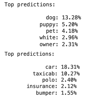
Two sample images — a golden retriever and a 2006 Toyota Camry — alongside their respective descriptions according to CLIP. The cosine similarity of the first image relative to the prompt “a golden retriever” is 0.2690, compared to 0.1586 for the second image.
In order to get a sense of where the solution might exist relative to our starting point, we’d like all operations involved in the process of computing this similarity score to be differentiable. That way, we’ll be able to follow the gradient of the function and use it to update our image at each step. To achieve our goals within a limited two-week timeframe, we desire rasterizers built on simple but powerful frameworks that would allow for as rapid iteration as possible. As such, PyTorch-based differentiable renderers like diffvg (2D) and Nvdiffrast (3D) provide the machinery to relate image embeddings with the parameters used to draw our primitives to the screen: we’ll be making extensive use of both throughout this project.
2D Shape Optimization
We started by looking at the 2D case, taking this paper as our basis. In this paper, the authors propose CLIPDraw: an algorithm that creates drawings from textual input. The authors use a pre-trained CLIP language-image encoder as a metric for maximizing the similarity between the given description and a generated drawing. This idea is similar to what our project hopes to accomplish, with the main difference being that CLIPDraw operates over vector strokes. We tried a couple of methods to make the algorithm more geometrically aware, the first of which is some data augmentations.
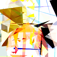
By default, the optimizer has too much creative leeway to interpret which images match our text prompt, leading to some borderline incomprehensible results. Here’s an example of a result that CLIP identifies as a “golden retriever” when left to its own devices:
Prompt = “a golden retriever” after 8400 iterations
Here, the optimizer gets the general color palette right while missing out completely on the geometric features of the image. Fortunately, we can force the optimizer to approach the problem in a more comprehensive manner by “augmenting” (transforming) the output at each step. In our case, we applied four random perspective & crop transformations (as do the authors of CLIPDraw) and a grayscale transformation at each step. This forces the optimizer to imitate human perception in the sense that it must identify the same object when viewed under different ambient conditions.
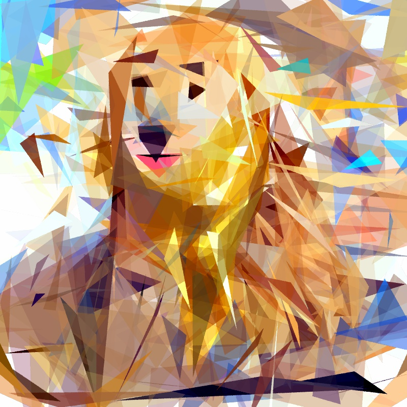
Fortunately, the introduction of data augmentations produced near-instant improvements in our results! Here is a taste of what the neural network can generate using triangles:
Prompt = “a Golden Retriever”Prompt = “a lighthouse”
Generating Meshes
In addition to manipulating individual shapes, we also tried to generate 2D triangular meshes using CLIP and diffvg. Since diffvg doesn’t provide automatic support for meshes, we circumvented this problem using our own implementation where individual triangles are connected to form a mesh. We started our algorithm with a simple uniform randomly-colored triangulation:
Initial mesh
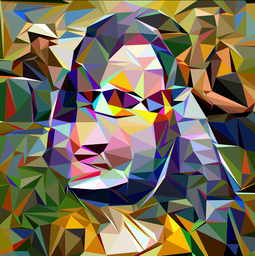
Simply following each step in the gradient direction could change their positions individually, destroying the mesh structure. So, at each iteration, we merge together vertices that would have been pushed away from each other. We also prevent triangles from “flipping”, or changing orientation in such a way that would produce an intersection with another existing triangle. Two of the results can be seen below:
Prompt = “Monalisa”Prompt = “Batman”
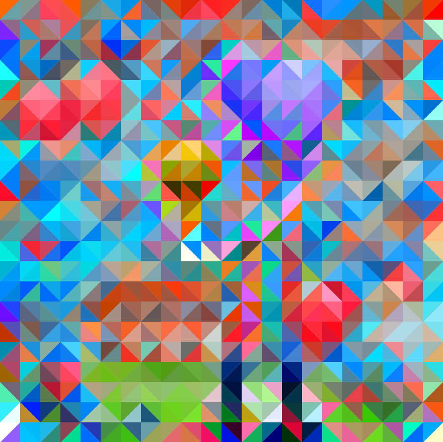
Throughout this process, we introduce and subsequently undo a lot of changes, making the process inefficient and the convergence slow. Another nice approach is to modify only the colors of the triangles rather than their positions and shapes, allowing us to color the mesh structure like a pixel grid:
Prompt = “Balloon” without changing triangle positions
Non-differentiable Operations and the Evolutionary Approach
Up until this point, we’ve only considered gradient descent as a means of solving our central optimization problem. In reality, certain operations involved in this pipeline are not always guaranteed to be differentiable, especially when it comes to rendering. Furthermore, gradient descent optimization narrows the range of images that we’re able to explore. Once a locally optimal solution is found, the optimizer tends to “settle” on it without experimenting further — often to the detriment of the result.
On the other end of the “random-deterministic” spectrum are evolutionary models, which work by introducing random changes at each step. Changes that improve the result are preserved through future steps, whereas superfluous or detrimental changes are discarded. Unlike gradient descent optimization, evolutionary approaches are not guaranteed to improve the result at each step, which makes them considerably slower. However, by exploring a wider set of possible changes to the images, rather than just the changes introduced by gradient descent, we gain the ability to explore more images.
Though we did not tune our evolutionary model to the same extent as our gradient descent optimizer, we were able to produce a version of the program that performs simple tasks such as optimizing with respect to the overall image color.
Prompt = “red” after 0 and 60 iterations
3D Shape Optimization
Moving into the third dimension not only gives us a whole new set of geometric primitives to play with, but also introduces fascinating ideas for image augmentations, such as changing the position of the virtual camera. While Nvdiffrast provides a powerful interface for rendering in 3D with automatic differentiation, we quickly discovered that we’d need to implement our own geometric framework before we could test its capabilities.
Nvdiffrast’s renderer is very elegant in its design. It needs only a set of triangles and their indices in addition to a set of vertex colors in order to render a scene. Our first task was to define a set of geometric primitives, as Nvdiffrast doesn’t provide out-of-the-box support for anything but triangles. For anyone familiar with OpenGL, creating an elementary shape such as a sphere is very similar to setting up a VBO/EBO. We set to work creating classes for a sphere, a cylinder, and a cube.
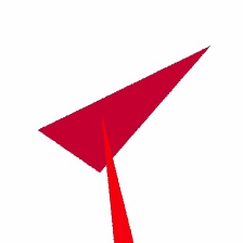
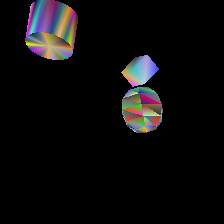
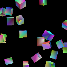
Random configuration of geometric primitives — a cube, a cylinder, and a sphere — rendered with Nvdiffrast. One example of an input to our algorithm.
Because the input to Nvdiffrast is one contiguous set of triangles, we also had to design data structures to mark the boundaries between discrete shapes in our triangle list. We did not want the optimizer to operate erratically on individual triangles, potentially breaking up the connectivity of the underlying shape: to this end, we devised a system by which shapes could only be manipulated by a series of standard linear transformations. Specifically, we allowed the optimizer to rotate, scale, and translate shapes at will. We also optimized according to vertex colors as in our previous 2D implementation.
With more time, it would have been great to experiment with new augmentations and learning rates for these parameters: however, setting up a complex environment like Nvdiffrast takes more time than one might expect, and so we have only begun to explore different results at the writing of this blog post. Some features that show promising outcomes are color gradient optimization, as well as the general positioning of shapes:
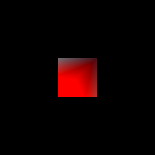
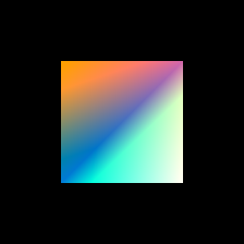
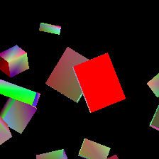
Prompt = “red”Prompt = “rainbow”prompt = “a centered red square” (before and after optimization)
Conclusion
Working on this project over the last few weeks, we saw that it is possible to achieve a lot with neural networks in a relatively short amount of time. Through our exploration of 2D and 3D cases, we were able to generate some early but promising results. More experiments are needed to test the limits of our model, especially with respect to the assembly of complex 3D scenes. Nonetheless, this method of using geometric primitives to synthesize images seems to have great potential, with a number of artistic applications making themselves evident through the results of our work
By Abraham Kassahun, Dimitry Kachkovski, Hongcheng Song, Shaimaa Monem
Introduction
It has been two weeks of the projects phase in SGI and our team has been working under the guidance of David Levin and Rohan Sawhney on a very interesting approach to solving differential equations using Mixed Finite Element Method.
In the beginning we were looking at how general Finite Element Methods (FEM) are used to solve the 2D Screened Poisson Equation (and later on a 3D one). First and foremost, we need to understand what FEM is. It is a discretization method that allows us to accurately solve differential equations. It allows us to break up a large system into simpler finite parts (in our case – triangles), and to make certain assumptions over these finite elements that help find a feasible solution.
If we look into the very simple case of only one triangle mesh, then given 3 vertices \(v_1, v_2, v_3\) that form this triangle, we attach a value of a function \(u\) at each of them (that is \(u(\textbf{v}_1),u(\textbf{v}_2),u(\textbf{v}_3)\)are known). To get the value of \(u(\textbf{v})\), for a point \(\textbf{v}\) inside the triangle, we can use various ways of interpolating between the 3 given values. Linear interpolations are often very useful for simulation, and we can use for instance barycentric coordinates as a way to interpolate these values.
A variation of the FEM method that we are exploring is called Mixed FEM. Its main idea is the introduction of supplementary independent variables that create additional constraints on the system. Mixed finite element method can precisely solve some very complex PDEs, while the ultimate goal of utilizing it in our project is to provide another more flexible skinning strategy, which automatically tunes deformation parameters to triangles by artist specified controls, while paving the way to an optimized version of the solver via the Adjoint Method.
Screened Poisson Equation
Figure 1. Screened Poisson equation solve over a 2D mesh with animated alpha parameter. (Credit: Abraham Kassahun Negash)
To understand how mixed FEM works, we first applied it to the heat equation. It turns out that it doesn’t have any advantages when applied to the heat equation, but it was a good pedagogical detour to understand how it works exactly. The heat equation is a type of Poisson equation described as:$$\Delta u = f$$ If solved as is, the resulting equation will not have a unique solution due to the absence of a Dirichlet boundary condition. Instead we modified the equation slightly by including an \(\alpha u\) term which allows the equation to be solved without explicitly giving any boundary conditions in MATLAB. $$\Delta u – \alpha u = f$$ This equation is also called the screened Poisson equation. We can solve for \(u\) by minimizing the following energy. $$E(u) = \frac{1}{2}\int_{\Omega}||\nabla u||^2 \,d\Omega + \frac{1}{2}\int_{\Omega} \alpha ||u||^2 \,d\Omega – \int_{\Omega} fu \,d\Omega$$ Where \(\Omega\) is our domain of interest. We can define \(u\) as a vector of values evaluated at the vertices of a triangle mesh. Then the equation can be discretized by writing \(u\) as the weighted average of vertex values. $$u(x) = \sum_{i=1}^3{\phi_i (x) u_i}$$ Where \(\phi_i (x)\) are the shape functions we use to interpolate \(u\) inside the triangle. We are going to let \(u\) be piecewise linear over our mesh by choosing linear shape functions. Thus the gradient of \(\phi\) is constant inside the triangle. Substituting into \(u\) and performing the integration we get the following expression. $$E(u) = \frac{1}{2}u^T G^T W G u + \frac{1}{2}\alpha u^T M u – u^T M f$$ Where:
\(G\) is the gradient matrix defined over the mesh
\(W\) is the weight matrix resulting from integrating \(\nabla u\) over faces
\(M\) is the mass matrix resulting from integrating functions over vertices
\(G\) is the gradient operator over the mesh and only depends on the vertex positions. The mass and weight matrices can be taken as identity by assuming a uniform mesh of equal triangles. It can be seen that the term with an \(\alpha\) acts the potential energy of a spring penalizing deviation of \(u\) from 0, thus preventing the solution from blowing up. The solution therefore reduces to $$E(u) = \frac{1}{2}u^T G^T G u + \frac{1}{2}\alpha u^T u – u^T f$$
To solve for \(u\) we formulate an optimization problem in a discrete form over some finite cells of a given surface, that is we build a Finite Element system and find the minimizer as follows:
$$u^* = \arg \min_{u}(\frac{1}{2} u^T G^T G u + \frac{1}{2} \alpha u^T u – u^T f)$$
Finally, to minimize the above system with the standard FEM, we must take the derivative of the function w.r.t. \(u\), and since the system is quadratic, setting the result to zero and solving for \(u\) will yield the answer. That is if we define the energy as $$E(u)=\frac{1}{2}u^T G^T G u + \frac{1}{2}\alpha u^T u – u^T f)$$ then we compute the gradient $$\nabla_u{E}=G^T G u + \alpha u – f =0$$ and we get $$G^T G u + \alpha u = f\\ (G^T G + \alpha I)u=f\\ u=(G^T G + \alpha I)^{-1} f$$
This means that the discrete solution can be computed through a linear system solution.
Mixed FEM
Figure 2. Mixed FEM solution of the ARAP energy by rotating a single triangle. (Credit: Shaimaa Monem)
As mentioned in the introduction, the main idea behind Mixed FEM is to introduce an additional independent variable that we solve for to allow us to optimize the search for the full solution to our system. That is, we will make everything much more complicated so as to make it easier later on! Yay!
We introduce such a variable by taking a part of the original energy equation \(E(u)\), and setting a constraint. That is, we want to reformulate the original minimization as $$g^*,u^* = \arg \min_{u,g}(\frac{1}{2} g^T g + \frac{1}{2} \alpha u^T u – u^T f)\\ s.t. \ Gu-g=0$$
The idea definitely feels awkward at first. But what we are looking to do is to define \(Gu\) as some variable that is independent of \(u\) itself, but that constrains the system for \(u\). Think of how the search for \(u\) was like turning some dials, and \(Gu\) was another dial that would turn as you try different settings for \(u\). Our goal is to separate that connection so that we can search for both independently, with that search governed by the established rule aka. our constraint.
To solve the newly emergent constrained optimization we use the method of Lagrange Multipliers and formulate our system as: $$\mathcal{L}{g^*,u^*,\lambda}=\arg \max_{\lambda} \min_{g^*,u^*}E + \lambda^T(Gu-g)\\ \mathcal{L}{g^*,u^*,\lambda}=\arg \max_{\lambda} \min_{g^*,u^*} \frac{1}{2} g^T g + \frac{1}{2} \alpha u^T u – u^T f + \lambda^T(Gu-g) $$
Now, we just need to take the gradient w.r.t. each of the variables, set them as before to 0, and solve for our 3 variables! That gets us: $$ \nabla_g=g-\lambda=0\\ \nabla_u=\alpha u – f + G^T \lambda=0\\ \nabla_{\lambda}=Gu-g=0$$
These 3 conditions that we got are known as Karush-Kuhn-Tucker (KKT) conditions. Using them we formulate a larger system that we solve: $$\begin{bmatrix} I & 0 & -I \\ 0 & \alpha I & G^T \\ -I & G & 0 \end{bmatrix} \begin{bmatrix} g\\ x\\ \lambda \end{bmatrix} = \begin{bmatrix} 0\\ f\\ 0 \end{bmatrix}$$
Solving this system will give us the solution that we are after.
Now this alone is obviously not a way to speed our solution up. However, the Mixed FEM formulation allows us to combine it with a numerical method known as the Adjoint Method, which in turn will indeed speed up the whole system. It also allows us to leverage certain aspects of deformation energies and their formulations which avoids such heavy handed computations as SVDs.
But before we get there, let’s move away from the toy problem, and consider how our mesh will deform.
As-Rigid-As-Possible (ARAP) Energy
Figure 3. A sine-based animation using Automatic Skinning using Mixed FEM. (Credit: Dimitry Kachkovski)
Deformation of elastic objects can be described using various different models. The one we consider is known as the As-Rigid-As-Possible model (Sorkine and Alexa, 2007).
ARAP is a powerful energy term which is invariant to rigid transformations, and it is designed to measure deformation in our system setting clearly, which has the form: $$E(F) = \| S – I \|_{F}^2$$ Where \(F\) represents the total transformation while \(S\) is a parameter unrelated to rigid transformation, which can be generated from polar decomposition from \(F\) using the relation \(F = RS\), where \(R\) is a rigid transformation. Therefore, energy is only dependent on non-rigid transformation, which has a global minimum at Identity. In this case, \(E(R) = 0\) and \(E(RS) = E(S)\). Instead of finding \(S\) through decomposition every time, what Mixed FEM allows us to do is to let \(S\) be an independent variable and enforce the relation \(F = RS\) with a constraint. Therefore, \(E\) can now be written as:$$E(S) = \| S – I \|_{F}^2$$
Using second-order Taylor expansion, ARAP energy takes the following form: $$E(S) = \frac{1}{2}S^THS + G^TS$$Where \(H\) and \(G\) are Hessian and gradient matrices, respectively.
Any rigid transformation exerted on triangle mesh will result in zero ARAP energy, but for any non-rigid deformation on triangle mesh, ARAP will clearly generate the corresponding energy. For example, in our gingerBrad man example, we pin down a rotation for a triangle; hence, the only possible situation to keep ARAP energy be zero is forcing all rotations of other triangles to be the same as the pinned one. You can imagine that if one of those triangles does not conform to the same rotation, non-rigid deformation will be generated in that triangle, leading to the growth of ARAP energy. So, ARAP skinning energy is indeed measuring the difference of energy between the current system state and the As-Rigid-As-Possible state with two boundary conditions, and the current state will finally reach the As-Rigid-As-Possible state by the optimizer.
Yoga Performance with Adjoint Method
1.1 Motivation and task formulation
Assuming we have a physics-based animation scene that we would love to visualize, we always start from a the continuous setting, then we choose a discretization scheme that allows us to write a piece of code to simulate our animations, we then pick our favorite programming language and turn the discrete model into a script that our computers can understand and deal with. If we are animating a character, then we would like it to match a specific behavior that is visually appealing, for example a special yoga pose. Well, assuming our character is sportive and flexible, then our simulator might do a good job imitating the desired behavior, if we define flexibility and athletic ability as parameters and feed them to our model. And we can see that in order to achieve successful animation we required three ingredients:
Discrete model simulating our object’s animations,
Target behavior for the object,
Input parameters tuning the object’s properties.
Sounds simple enough! But it implies that we need to know everything beforehand, which is not the case with movie character animation. We might know our target behavior but we do not know the parameters values that take us to this specified behavior, for instance how do we tune flexibility for gingerBrad so that it can do yoga without breaking?
We can express this yoga pose as a desired deformation through a deformation energy which happens to be the well known and previously mentioned ARAP energy. Therefore, we can basically translate this into an optimization task to find, for instance, the threshold \(p^{\star}\) of the flexibility parameter that is enough to reach the yoga pose, $$p^{\star} = \arg \min_{p} \ E_{ARAP}(p)$$
If you have been to a yoga class, then you have heard your instructor say – “Keep your toes forward and your heels down to the floor, straight back…” – and so on! Well, this is one of the powers that comes with using skinning technique: we can easily pin gingerBrad’s feet to the ground using handles, as follows: $$p^{\star} , x^{\star} = \arg \min_{p,x} \ E_{ARAP}(p) + \frac{k}{2} \| P x – x_{pinned} \|^2 $$
This means that we can optimize not only over \(p\) but also over all vertex positions \(x\) of the gingerBrad mesh, and we get \(x^{\star}\) the optimal position that is as close as possible to the pose we want, with heals \(x_{pinned}\) pinned to the ground. In the equation above \(P\) is a pinning matrix that selects from \(x\) only the verts to which we assign boundary conditions (here simply pinning!).
So far so good. Now let us imagine a more complex scenario where it is hard to exactly define what that target pose would look like. To picture this situation, let us assume that the gingerBrad character actually got a job as a yoga instructor, and now many characters are standing behind copying the yoga moves! Well, realistic experience tells us that they will not all reach the same exact final yoga pose, as they have different body properties reflected through a wide range of flexibility parameter values, and for the sake of our health and sanity we want to avoid solving a separate problem for each participant, especially ifgingerBrad is a very beloved famous coach and his class is always full :-)
We know that we want all of them to go as close as they could to a specific yoga pose, so let us assume, for simplicity, that we want them to rotate their bodies while still standing on the ground We can represent this very special yoga pose with a rotation matrix \(R\). But we can clearly see that the way this rotation task goes for each of them depends on their shapes, i.e. positions \(x\), and properties, or, as we call it, parameters \(p\), which in turn depend on the assigned rotation, meaning we have \(x(R)\) and \(p(R)\).
To find the rotation that each of them can achieve, we must formulate another optimization task:
$$ R^{\star} = \arg \min_{R} \ E_{ARAP}(p) + \frac{k}{2} \| P x – x_{pinned} \|^2 + \| R – R_{pinned} \|^2$$
Where \(R_{pinned}\) makes sure that our animated characters perform rotation around their pinned vertices, for consistency.
Now arises a huge EXISTENTIAL QUESTION, if \(R\) depends on\(p\) and \(x\) which in return are functions of \(R\), how can we compute any of them??
1.2 Apply Adjoint Method
Well basically the adjoint method is the solution to this problem, and we will go through this step by step.
First, remember that finding \(R^{\star}\) is our ultimate goal, as we want to visualize the yoga poses for all our animated characters and visualize how they perform. We ask ourselves, what do we need to solve the second optimization to compute \(R^{\star}\)? And the simple answer is that we need to find the critical points to the gradient $$E(R)= E_{ARAP}(p)+ \frac{k}{2} \| P x – x_{pinned} \|^2 + \| R – R_{pinned} \|^2\\ \frac{d E(R)}{d R} = \frac{\partial x}{\partial R} \frac{\partial E(R)}{\partial x} + \frac{\partial p}{\partial R} \frac{\partial E(R)}{\partial p} + \frac{\partial E(R)}{\partial R} = 0$$ While computing this gradient requires \(\frac{\partial x}{\partial R}\) and \(\frac{\partial p}{\partial R}\) as \(x\) and \(p\) are functions of \(R\).
Second, we can actually exploit the first optimization problem to compute \(\frac{\partial x}{\partial R}\) and \(\frac{\partial p}{\partial R} \).
Let’s perform the steps for a special parameter and explain more. We want \(p\) to relate to the deformation \(F\) which expresses the deformed state. We can specifically use the polar decomposition and write \(F\) as a decomposition of a rotation matrix \(R\) and a symmetric matrix \(S\), i.e. \(F = R S\). Remember that we are optimizing \(R\), therefore we are left with \(S\) to pick as our parameter. Moreover, we can find a linear operator called deformation gradient \(B\) that represents this deformation and basically takes our character from its rest reference pose to the deformed yoga performance pose. This gives us a constraint \( B x = RS\) which leads to the following constrained optimization problem
$$ S^{\star} , x^{\star} = \arg \min_{S,x} \ E_{ARAP}(S) + \frac{k}{2} \| P x – x_{pinned} \|^2 $$
Such that \( B x = R S\) (note: I am skipping technical details for simplicity!)
Now the latest constrained optimization task can be happily solved through a Lagrangian energy, actually arising from a mixed FEM problem as explained previously.
$$L(S, x, \lambda) = E_{ARAP}(S) + \frac{k}{2} \| P x – x_{pinned} \|^2 + \lambda (Bx – RS)$$
And like we saw in the very beginning of the report we proceed with computing the gradients of \(L(S, x, \lambda)\) w.r.t. its three different variables and formulate a linear system to solve
$$\nabla_S L = HS + g^T – R^T \lambda = 0\\ \nabla_x L = \frac{k}{2} P^TP + B^T \lambda = 0\\ \nabla_{\lambda} L = B x- R S = 0$$
We rewrite this as \(A y = b \) , where \(A\) is the KKT matrix and \(y = (S^{\star}, x^{\star} , \lambda)^T\) is the solution for our first optimization problem.
Third, we can extract \(S^{\star}\) and \(x^{\star}\) from \(y\) and fix them in \(E(R)\), which leads to $$E(R)= E_{ARAP}(S^{\star})+ \frac{k}{2} \| P x^{\star} – x_{pinned} \|^2 + \| R – R_{pinned} \|^2$$
Fourth, now we can see that, actually, the derivatives that we require are \(\frac{\partial x^{\star}}{\partial R}\) and \(\frac{\partial S^{\star}}{\partial R}\) , which can be computed by differentiating \(y\) , i.e. \(\frac{\partial y}{\partial R} = (\frac{\partial S^{\star}}{\partial R} , \frac{\partial x^{\star}}{\partial R} , 0)^T\), given by $$\frac{\partial y}{\partial R} = \frac{\partial A^{-1}}{\partial R} \ b\\ \frac{\partial y}{\partial R} = – A^{-1 } \ \frac{\partial A}{\partial R} A^{-1 } \ b$$
Finally, now that we have \(\frac{\partial x^{\star}}{\partial R}\) and \(\frac{\partial S^{\star}}{\partial R}\), we can basically substitute them into the energy derivative \(\frac{d E(R)}{d R}\) and find \(R\) as the critical point, Woooh!
One more important aspect that we need to take care of is to make sure that \(R\) stays still as a rotation matrix along the optimization task, for this reason, we explicitly write \(R\) as an orthogonal 2D matrix $$R(\theta) = \begin{bmatrix} cos \theta & sin \theta \\ – sin \theta & cos \theta \end{bmatrix} $$ And express our energy in terms of \(\theta\) instead, as follows $$\frac{d E(\theta)}{d \theta} = \frac{\partial x}{\partial \theta} \frac{\partial E(x(\theta),p(\theta),\theta)}{\partial x} + \frac{\partial p}{\partial \theta} \frac{\partial E(x(\theta),p(\theta),\theta)}{\partial p} + \frac{\partial E(x(\theta),p(\theta),\theta)}{\partial \theta} = 0$$
All that is left is to give the solver of our choice an initial guess of the angle and let it run. And now we can find the yoga poses for all participants in the yoga class coached by gingerBread and render an animation if we want.
Figure 4. Manipulation of handles with Automatic Skinning using Mixed FEM. (Credit: Hongcheng Song)
Take away home: next time you go to Yoga class do not forget your Adjoint Method 🙂
1.3 Apply Adjoint Method to High Resolution Mesh
Even though the adjoint method is able to accelerate the optimization process of angles by analytical gradient, it is still an extremely expensive process to use for high resolution meshes. Therefore, we use average biharmonic weights and optimized angles of blue noise sample points to approximate the final result. This approximation propagates those optimal solutions to all triangles by introducing biharmonic weights, allowing a smooth angle interpolation across the surface and reducing enormous calculation expenses required for optimizing all triangles.
Where \(f\) is the number of triangle faces, \(h\) is the number of sample points. \(W_{i, j}\) is the biharmonic weights of a triangle with respect to each sample point, and \(\theta_j\) is the optimized solution of sample points.
References (APA style):
Sorkine, O., & Alexa, M. (2007, July). As-rigid-as-possible surface modeling. In Symposium on Geometry processing(Vol. 4, pp. 109-116).