Butlerian concerns aside, neural networks have proven to be extremely useful in doing everything we couldn’t think was to be done in this century; extremely advanced language processing, physically motivated predictions, and making strange, artful images using the power of bankrupt corporate morality.
Now, I’ve read and seen a lot of this “stuff” in the past, but I never really studied it, in-depth. Luckily, I got put with four exceedingly capable people in the area, and now manage to write a tabloid on the subject. I’ll write down the very basics of what I learned this week.
Taylor’s theorem
Suppose we had a function \( f : F \rightarrow L \) between the feature space \(F\) and a label space \(L\), both of these spaces are composed of a finite set of data points \( x_i \) and \( y_i \), we’ll put them into a dataset \(\mathfrak{D} = \{(x_i, y_i,) \}^N_{i=1} \). This function can represent just about anything as long as we’re capable of identifying the appropriate labels; images, videos and weather patterns.
The issue is, we don’t know anything about \(f\), but we do have a lot of data, so can we construct a arbitrarily good approximation \( f_\theta \) that functions a majority of the time? The whole field of machine learning asks not only if this is possibly, but if it is, how does one produce such a function, and with how much data?
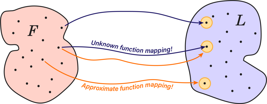
Indeed, such a mapping may be extremely crooked, or of a high-dimensional character, but as long as we’re able to build universal function approximators of arbitrary precision, we should, in principle, be able to construct any such function.
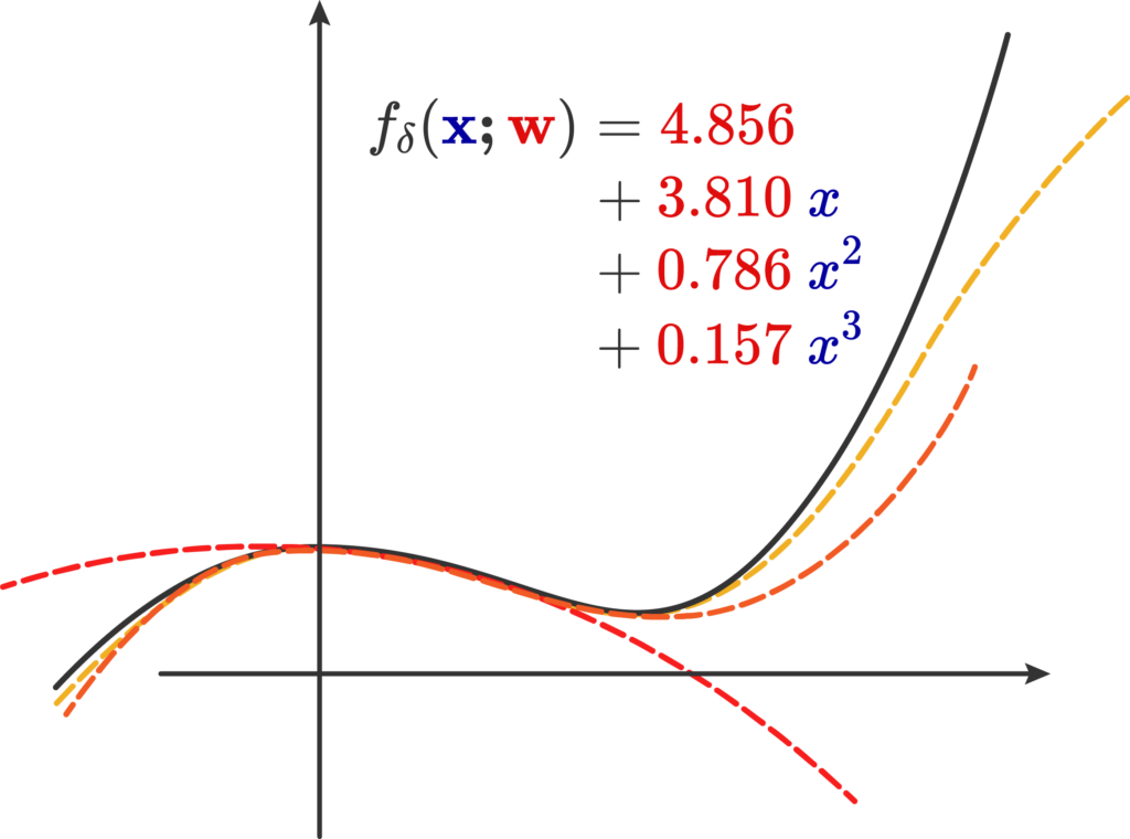
Naively, the first type of function approximator is a machine that produces a Taylor expansion; we call this machine \( f_\delta(\mathbf{x;w}) \) that approximates the real \( f(\mathbf{x})\). It contains the function input \( \mathbf{x}\), and a weight vector \(\mathbf{w}\) containing all of the coefficients of the Taylor expansion. We’ll call this parameter list the weights of the expansion.
Indeed, this same process can be taken up by any asymptotic series that converges onto the result. Now, what we’ve done is that we already had the function and wanted to find this approximation. Can we do the reverse procedure of acquiring a generic third degree polynomial: \[ f_\delta(x) = c_0 + c_1x + c_2 x^2 + c_3 x^3 \]
And then find the weights such that around the chosen point \( \mathbf{x} \) it fits with minimal loss? This question if of course, a extensively studied area of mathematically approximating/interpolating/extrapolating functions, and also the motivating factor for a NN, they’re effectively more complicated versions of this idea using a different method of fitting these weights, but it’s the same principle of applying a arbitrarily large number of computations to get to some range of values.
The first issue is that the label and feature spaces are enormously complicated, their dimensionality alone poses a formidable challenge in making a process to adjust said weights. Further, the structure in many of these spaces is not captured by the usual procedures of approximation. Taylor’s theorem, as our hanged man, is not capable of approximating very crooked functions, so that alone discards it, but
Thought(Thought(Thought(…)))

A neural network is the graphic representation of our neural function \(f_\theta\). We will define two main elements: a simple affine transform \(L = \mathbf{A}_i \mathbf{x} + \mathbf{b}_i \), and a activation function \( \sigma(L\), which can be any function, really, including a polynomial, but we often use a particular set of functions that are useful for NNs, such as a ReLu or a sigmoidal activation.
We can then produce a directed graph that shows the flow of computations we perform on our input \( \mathbf{x}\) across the many neurons of this graph. In this basic case, we have that the input \(x\) is feed onto two distinct neurons. The first transformation is \( \sigma_1(A_1x+b_1) \), whose result, \(x_1\), is feed onto the next neuron; the total result is a composition of the two transforms \(f \circ g = \sigma_2(A_2(f)+b_2 = \sigma_2(A_2(\sigma_1(A_1x+b_1))+b_2) \).
The total result of this basic net on the right is then \(\sigma_3(z) + \sigma_5(w) \), where \(w\) is the result of the transformations in the left, and \(z\) the ones on the right. We could do a labeling procedure and see then that the end result is of the form of a direct composition across the right layer of the affine transforms \((A, B, C)\) and activation functions \( (\sigma_1, \sigma_2, \sigma_3 \), and of the left hand side affine transforms \( (D, E, F) \) and functions \( (\sigma_4, \sigma_5, \sigma_6 ) \), which provides a 12-dimensional weight vector \( \mathbf{w} \):
\[ f_\theta(\mathbf{x;w}) = (\sigma_3\circ C \circ \sigma_2 \circ B \circ \sigma_1 \circ A) + (\sigma_6 \circ F \circ \sigma_5 \circ E \circ \sigma_4 \circ D) \]
Once again, the idea is that we can retrofit the coefficients of the affine transforms and activation functions to express different function approximations; different weight vectors yield different approximations. Finding the weights is called the training of the network and is done by an automatic process.
A feed forward NN is a deep, meaning it has more than intermediate layer, neural function \( f_\theta(\mathbf{x;w}) \) that, given some affine transformation \(f\) and activation function \(f\), is defined by:
\[ f_\theta(\mathbf{x;w}) = f_{n+1} \circ \sigma _n \circ f_n \circ \cdots \sigma_1\circ f_1 : \mathbb{R}^{n} \rightarrow \mathbb{R}^{n+1} \]
Here we see a basic FF neural function \( f_\theta (\mathbf{x, w}) \) and its corresponding neural network representation; it has a depth of 4 and a width of 3. The input \( x\) is feed into a singular neuron, that doesn’t change it, and its then feed to three distinct neurons, each with its own weights for the affine transformation, and this all repeats until the last neuron. All of them have the same underlying activation function \( \phi\):
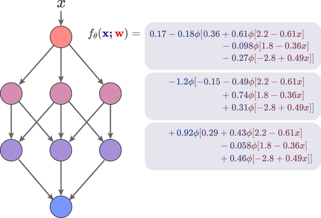
If we actually go out and compute this particular neural function using \( \phi \) as the sigmoid function, we get the approximation of a sine wave. Therefore, we have sucessfully approximated a low dimensional function using a NN How did we, however, get these specifics weights? By means of gradient descent. Maybe I’ll write something about the trainings of NNs as I learn more about them.
Equivariant NNs
Now that we approximated a simple sine wave, the obvious next step is the three dimensional reconstruction of a mesh into a signed distance function.
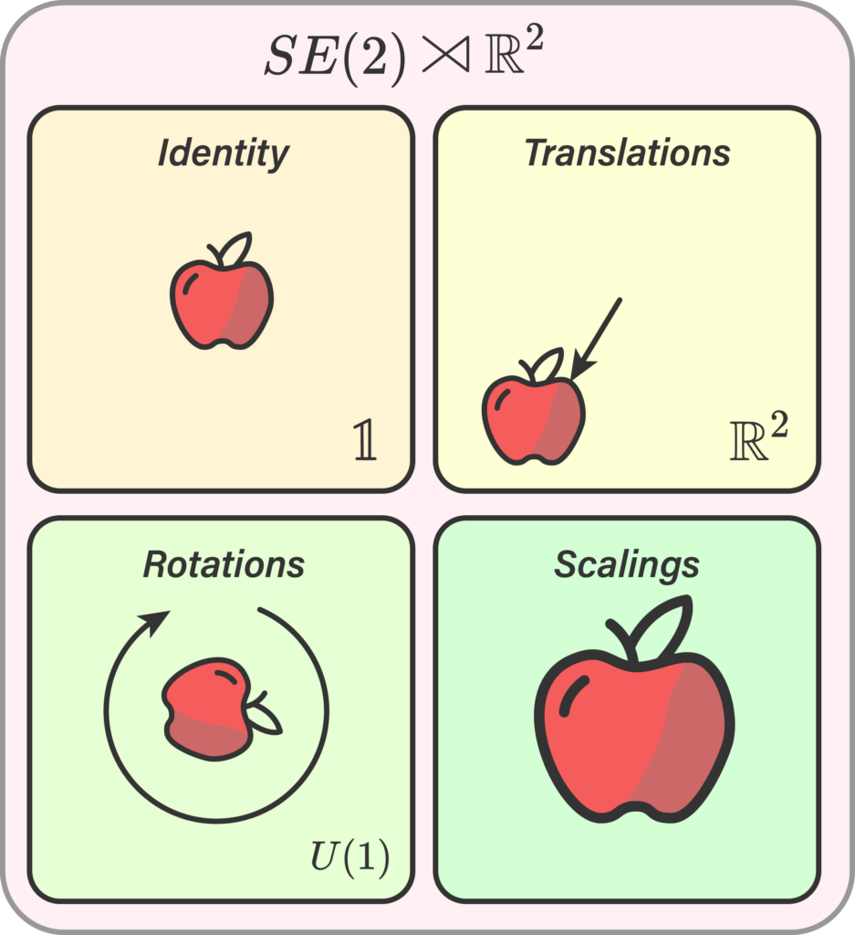
But since I don’t actually know the latter, I’ll go to the non-obvious next step of looking at the image of an apple. If we were to perform a transformation on said apple as either a translation, rotation, or scaling, ideally our neural network should be able to still identify the data as an apple. This means we somehow need to encode the symmetry information onto the weights of the network. This breeds the principle of an equivariant NN, studied in the field of geometrical deep learning.
I’ll try to study these later to make more sense about them as well.