If you have an object which you would like to represent as a mesh, what measure do you use to make sure they’re matched nicely?
Suppose you had the ideal, perfectly round implicit sphere \( || \mathbf{x}|| = c\), and you, as a clever geometry processor, wanted to make a discrete version of said sphere employing a polygonal mesh \( \mathbf{M(V,F)}\). The ideal scenario is that by finely tessellating this mesh into a limit of infinite polygons, you’d be able to approach the perfect sphere. However, due to pesky finite memory, you only have so many polygons you can actually add.
The question then becomes, how do you measure how well the perfect and tessellated spheres match? Further, how would you do it for any shape \( f(\mathbf{x}) \)? Is there also a procedure not just for perfect shapes, but also to compare two different meshes? That was the objective of Nicholas Sharp’s research program this week.
The 1D Case
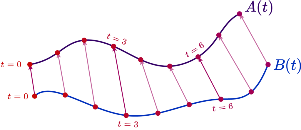
Suppose we had a curve \( A(t):[0,1] \rightarrow \mathbb{R}^n \), and we want to build an approximate polyline curve
\( B(t) \). We want to make our discrete points have the nearest look to our original curve \( A(t) \).
As such, we must choose an error metric measuring how similar the two curves are, and make an algorithm that produces a curve that minimizes this metric. A basic one is simply to measure the total area separating the approximate and real curve, and attempt to minimize it.
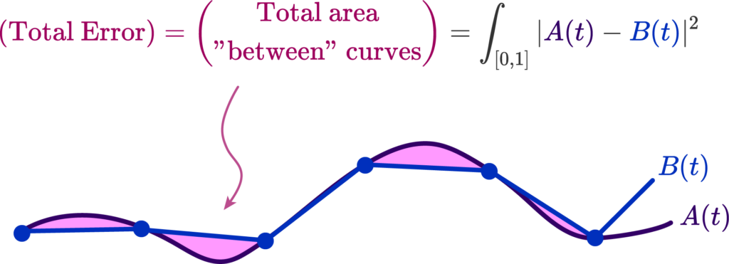
The distance between the polyline and the curve \( |A(t) – B(t)| \) is what allows us to produce this error functional, that tells us how much or how little they match. That’s all there is to it. But how do we compute such a distance?
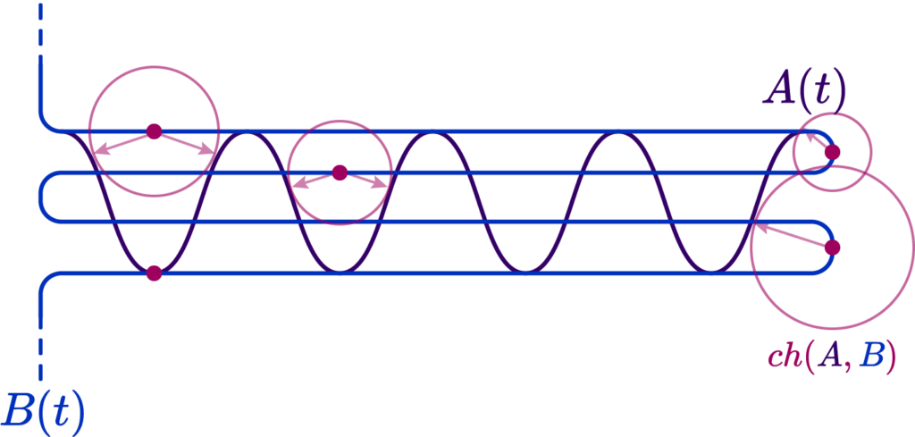
Well, one way is the Chamfer Distance of the two sets of points \( ch(A,B) \). It’s defined as the nearest point distance among the two curves, and all you need to figure it out is to draw little circles along one of the curves. Where the circles touch defines their nearest point!
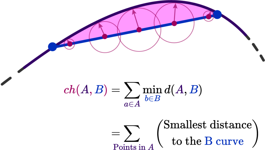
Here \( d(A,B) \) is just the regular Euclidean distance. Now we would only need to minimize a error functional proportional to \[ \partial E(A,B) = \int_{\gamma} ch(A,B) \sim \sum_{i=0}^n dL \ ch(A, B) = 0 \]
Well simple enough, but there’s a couple of problems. The first one is most evident: a “nearest point query” between curves does not actually contain much geometrical information. A simple counterexample is a spikey curve near a relatively flat curve; the nearest point to a large segment of the curve is a single peak!
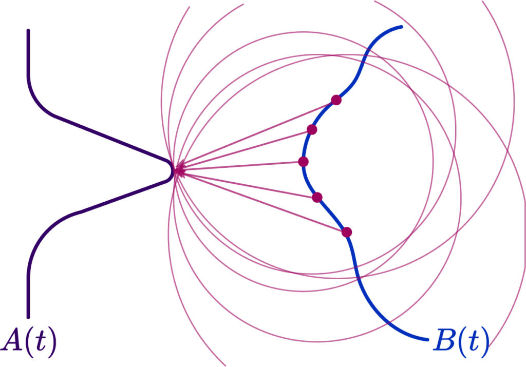
We’ll see another soon enough, but this immediately brings into question the validity of an attempted approximation using \( ch(A,B) \). Thankfully mathematicians spent a long time idly making up stuff, so we actually have a wide assortment of possible distance metrics to use!
Different error metrics
The first alternative metric is the classic Hausdorff Distance, defined as upper bound of the Chamfer distance. Along a curve, always picking the smallest distances, we can select the largest such distance.
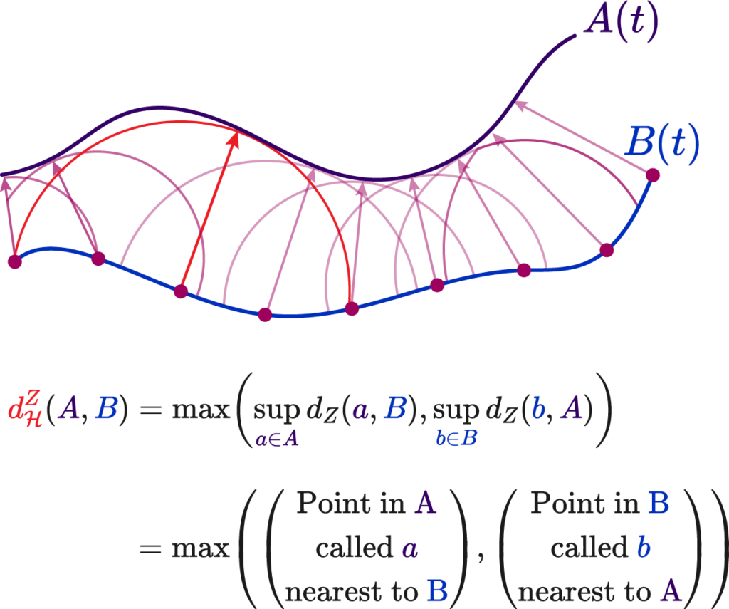
Where we to use such a value, the integral error would be akin to the mean error value, rather than the absolute total area. This does not fix our original shape problem, but it does facilitate computation!
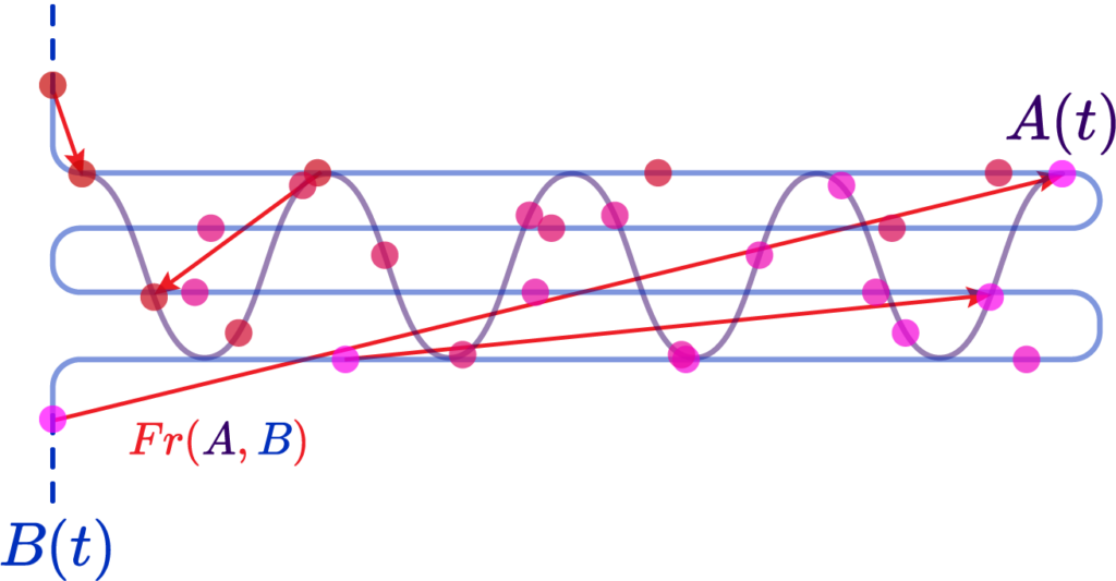
The last contender for our curves is the Fréchet Distance. It is relatively simple: you parametrize two curves \( A \) and \( B \) by some parameter \( t \) such that \(A(\alpha(t)) \) and \( B(\beta(t))\), you can picture it as time; it is always increasing. What we do is say that Fréchet distance \( Fr(A,B) \) is the instantaneous distance between two points “sliding along” the two curves:
We can write this as \[ Fr(A, B) = \inf_{\alpha, \beta} \max_{t\in[0,1]} d(A(\alpha(t)), B(\beta(t))) \]
This provides many benefits at the cost of computation time. The first is that it immediately corrects points from one of our curves “sliding back” as in the peak case, since it must be a completely injective function in the sense one point at some parameter \( t \) must be unique.
The second is that it encodes shape data. The shape information is contained in the relative distribution of the parametrization; for example, if we were to choose \( \alpha(t) \approx \ln t \), we’d produce more “control points” at the tail end of the curve and that’d encode information about its derivatives. The implication being that this information, if associated to the continuity \( (C^n) \) of the curve, could imply details of its curvature and such.
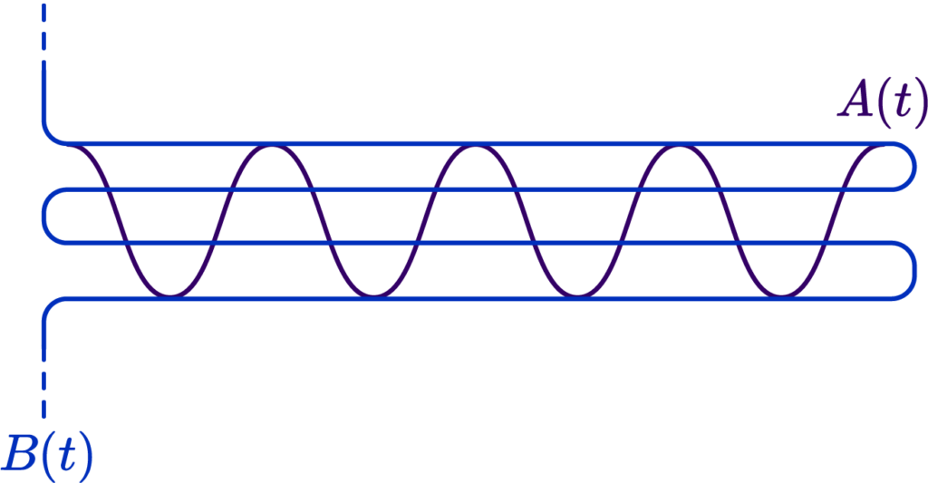
Here is a simple example. Suppose we had two very squiggly curves criss-crossing each other:
Now, were we to choose a Chamfer/Hausdorff distance variant, we would actually get a result indicating a fairly low error, because, due to the criss-cross, we always have a small distance to the nearest point:
However, were we to introduce a parametrization along the two curves that is roughly linear, that is, equidistant along arclenghts of the curve, we could verify that their Fréchet distance is very large, since “same moment in time” points are widely distanced:
Great!
The 2D case
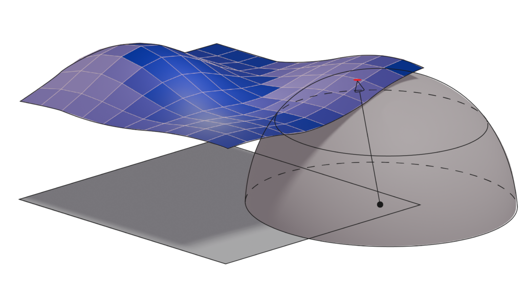
In our experiments with Nicholas, we only got as far as generalizing this method to disk topology, open grid meshes, and using the Chamfer approach to them. We first have a flat grid mesh, and apply a warp function \( \phi(\mathbf{x}) \) that distorts it to some “target” mesh.
def warp_function(uv):

    # input: array of shape (n, 2) uv coordinates. (n,3) input will just ignore the z coordinate

    ret = []
    for i in uv:
        ret.append([i[0], i[1], i[0]*i[1]])

    return np.array(ret)
We used a couple of test mappings, such as a saddle and a plane with a logarithmic singularity.
We then do a Chamfer query to evaluate the absolute error by summing all the distances from the parametric surface to the grid mesh. The 3D Chamfer metric is simply the nearest sphere query to a point in the mesh:
def chamfer_distance(A, B):
    ret = 0
    closest_points = []

    for a in range(A.shape[0]):
        min_distance = float('inf')
        closest_point = None
        for b in range(B.shape[0]):
            distance = np.linalg.norm(A[a] - B[b])
            if distance < min_distance:
                min_distance = distance
                closest_point = b
        ret += min_distance
        closest_points.append((a, A.shape[0]+closest_point))

    closest_points_vertices = np.vstack([A, B])
    closest_points_indices = np.array(closest_points)

    assert closest_points_indices.shape[0] == A.shape[0]
and closest_points_indices.shape[1] == 2
    assert closest_points_vertices.shape[0] == A.shape[0] + B.shape[0] and closest_points_vertices.shape[1] == A.shape[1]

    return ret, closest_points_vertices, closest_points_indices
Our main goals were to check if, as the base grid mesh was refined, the error diminished as the approximation increased in resolution, and to see if the relative angle of the grid mesh to the test function significantly altered the error.
The first experiment was validated quite successfully; besides perhaps very pathological cases, the error diminished as we increased the resolution:
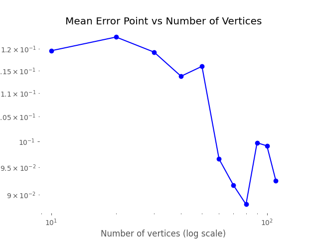
And the second one as well, but this will be discussed in a separate blog post.
Application Areas: Chamfer Loss in Action
In machine learning, a loss function is used to measure the difference (i.e. error) between the given input and the neural network’s output. By following this measure, it is possible to have an estimate of how well the neural network models the training data and optimize its weights with respect to this.
For the task of mesh reconstruction, e.g. reconstructing a surface mesh given an input representation such as a point cloud, the loss function aims to measure the difference between the ground truth and predicted mesh. To achieve this, the Chamfer loss (based on the Chamfer distance discussed above) is utilized.
Below, we provide a code snippet for the implementation of Chamfer distance from a widely adopted deep learning library for 3D data, PyTorch3D [1]. The distance can be modified to be used as single or bi-directional (single_directional) and by adopting additional weights.
def chamfer_distance(
    x,
    y,
    x_lengths=None,
    y_lengths=None,
    x_normals=None,
    y_normals=None,
    weights=None,
    batch_reduction: Union[str, None] = "mean",
    point_reduction: Union[str, None] = "mean",
    norm: int = 2,
    single_directional: bool = False,
    abs_cosine: bool = True,

):

    if not ((norm == 1) or (norm == 2)):

        raise ValueError("Support for 1 or 2 norm.")

    x, x_lengths, x_normals = _handle_pointcloud_input(x, x_lengths, x_normals)

    y, y_lengths, y_normals = _handle_pointcloud_input(y, y_lengths, y_normals)

    cham_x, cham_norm_x = _chamfer_distance_single_direction(
        x,
        y,
        x_lengths,
        y_lengths,
        x_normals,
        y_normals,
        weights,
        batch_reduction,
        point_reduction,
        norm,
        abs_cosine,
    )
    if single_directional:
        return cham_x, cham_norm_x

    else:
        cham_y, cham_norm_y = _chamfer_distance_single_direction(

            y,
            x,
            y_lengths,
            x_lengths,
            y_normals,
            x_normals,
            weights,
            batch_reduction,
            point_reduction,
            norm,
            abs_cosine,
        )

        if point_reduction is not None:
            return (
                cham_x + cham_y,
                (cham_norm_x + cham_norm_y) if cham_norm_x is not None else None,
            )
        return (
            (cham_x, cham_y),
            (cham_norm_x, cham_norm_y) if cham_norm_x is not None else None,

        )
When Chamfer is not enough
Depending on the task, the Chamfer loss might not be the best measure to estimate the difference between the surface and reconstructed mesh. This is because in certain cases, the \( k \)-Nearest Neighbor (KNN) step will always be taking the difference between the input point \( \mathbf{y} \) and the closest point \( \hat{\mathbf{y}}\) on the reconstructed mesh, leaving aside the actual point where the measure should be taken into account. This could lead a gap between the input point and the reconstructed mesh to stay untouched during the optimization process. Research for machine learning in geometry proposes to adopt different loss functions to mitigate this problem introduce by the Chamfer loss.
A recent work Point2Mesh [2] addresses this issue by proposing the Beam-Gap Loss. For a point \( \hat{\mathbf{y}}\) sampled from a deformable mesh face, a beam is cast in the direction of the deformable face normal. The beam intersection with the point cloud is the closest point in an \(\epsilon\) cylinder around the beam. Using a cylinder around the beam instead of a single point as in the case of Chamfer distance helps reduce the gap in a certain region between the reconstructed and input mesh.
The beam intersection (or collision) of a point \( \hat{\mathbf{y}}\) is formally given by \( \mathcal{B}(\hat{\mathbf{y}}) = \mathbf{x}\) and the overall beam-gap loss is calculated by:
\[ \mathcal{L}_b (X, \hat{\mathbf{Y}}) = \sum_{ \hat{y} \in \hat{Y}} |\hat{\mathbf{y}}-\mathcal{B}(\hat{\mathbf{y}})|^2 \]
References
[1] Ravi, Nikhila, et al. “Accelerating 3d deep learning with pytorch3d.” arXiv preprint arXiv:2007.08501 (2020).
[2] Hanocka, Rana, et al. “Point2mesh: A self-prior for deformable meshes.” SIGGRAPH (2020).
[3] Alt, H., Knauer, C. & Wenk, C. Comparison of Distance Measures for Planar Curves. Algorithmica
[4] Peter Schäfer. Fréchet View – A Tool for Exploring Fréchet Distance Algorithms (Multimedia Exposition).
[5] Aronov, B., Har-Peled, S., Knauer, C., Wang, Y., Wenk, C. (2006). Fréchet Distance for Curves, Revisited. In: Azar, Y., Erlebach, T. (eds) Algorithms
[6] Ainesh Bakshi, Piotr Indyk, Rajesh Jayaram, Sandeep Silwal, and Erik Waingarten. 2024. A near-linear time algorithm for the chamfer distance. Proceedings of the 37th International Conference on Neural Information Processing Systems.