SGI Fellows: Harini Rammohan, Ashlyn Lee, Diana Aldana Moreno, Ehsan Shams, Taylor Hospodarec
Project Mentor: Mikhail Bessmeltsev
SGI Volunteer: Daniel Perazzo
Raster vs Vector Images
Raster and vector graphics are two fundamental types of image representations used in digital design, each with distinct characteristics and applications. A raster image is a collection of colored pixels in a bitmap, making it well-suited for capturing detailed, complex images like photographs. However, raster graphics provide no additional information about the structure of the object they represent. This limitation can be problematic in scenarios where precision and scalability are essential. For example, representing an artist’s sketch as a raster image may result in jagged curves and the loss of fine details from the original sketch. In such cases, a vector graphics representation is preferred. Unlike raster images, vector graphics use mathematical equations to define shapes, lines, and curves, allowing unlimited scalability without losing quality. This makes vector graphics ideal for logos, illustrations, and other designs where clarity and precision are crucial, regardless of size.
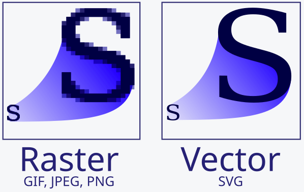
Image from https://en.wikipedia.org/wiki/Image_tracing
Bicubic Curves for Vectorization
In this project, we aimed to obtain a vector graphics representation of a given sketch in raster form using bicubic curves. A bicubic curve is a polynomial of the form

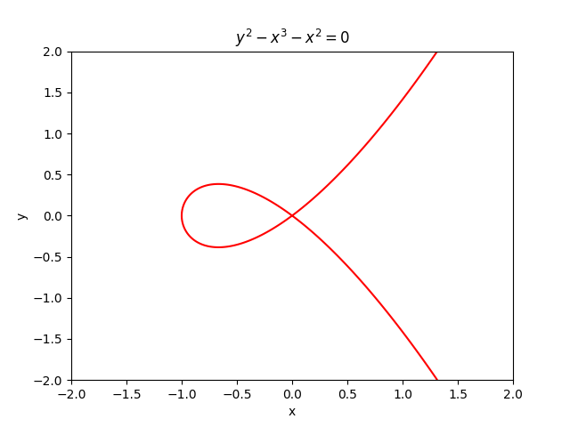
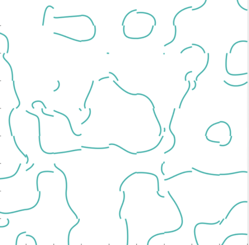
The value a bicubic function takes on a given grid cell is assumed to be uniquely determined by the value the function and its derivatives take at the vertices of the cell. Using bicubic curves allows us to more easily handle self-intersections and closed curves. Additionally, we can create discontinuities at the edges of grid cells by adding some noise to the given bicubic function. This will enable us to vectorize not only smooth but also discontinuous sketches.
Preliminary Work
During the first week of the project, we implemented the following using Python:
- For any given grid cell, given its size and the function value p(v) as well as the derivatives px(v), py(v), and pxy(v) at each vertex v, we reconstructed and plotted the unique bicubic function satisfying these values. This reduces to solving a system of sixteen linear equations, following the steps mentioned in the “Bicubic Interpolation” Wikipedia page {4}.
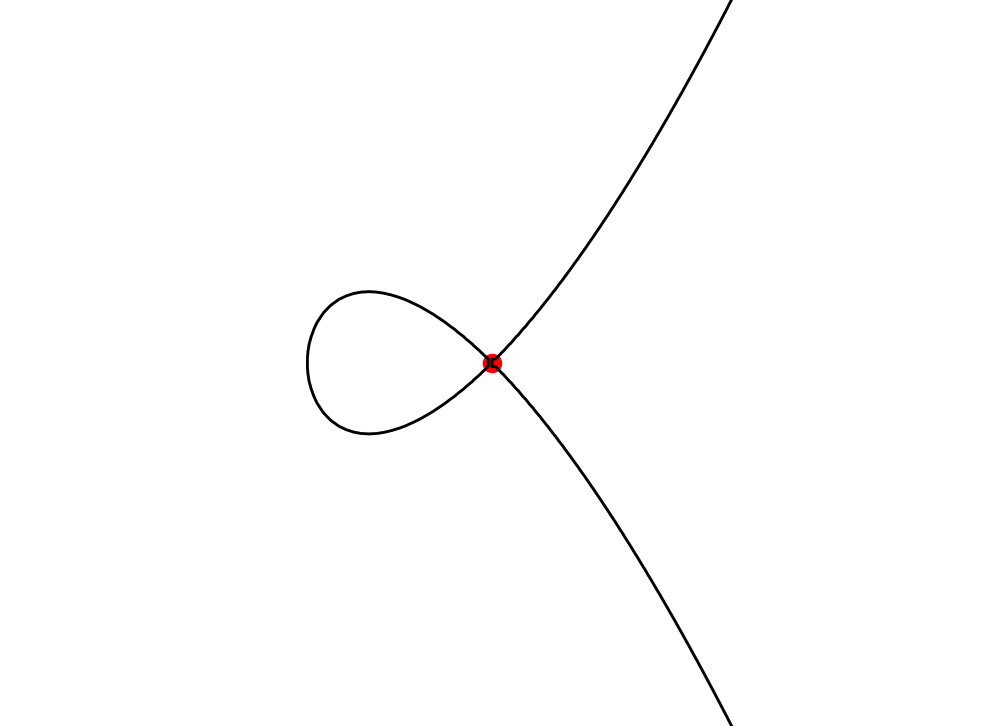
- We added noise to the bicubic functions in each cell to create discontinuities. We also found the endpoints of curves in the grid due to the discontinuities formed above.
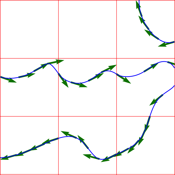
- At each point in the grid, we found the gradient of the bicubic functions using fsolve {5} and used them to plot the tangents at some points on the curves.
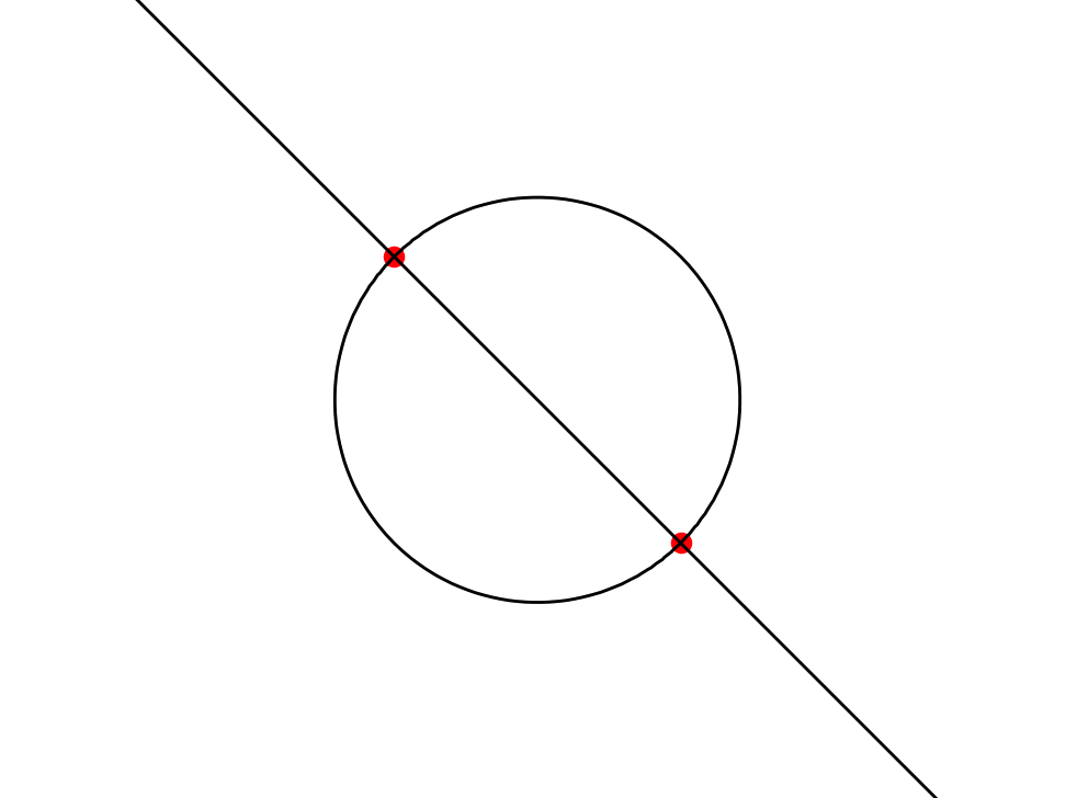
- We looked for self-intersections within a grid cell by finding saddle points of the bicubic function (such that the function value is 0 there). If the function is factorizable, it suffices to find the points of intersections between the 0-levels of two or more factors. Here too, we used fsolve.
Optimization and Rendering
Vectorization
During the second week of the project, I attempted to vectorize the bitmap image by minimizing a function known as the L2 loss.
The L2 loss between the predicted and target bitmap images is computed as the sum of the squared differences for each pixel. To account for this, I gave the bicubic curves some thickness by replacing the curve Z = 0 (here Z = p(x, y) is a bicubic function) in each grid cell with the image of the function e-Z². This allowed me to determine the color at each point in the grid, defining the color of each pixel as the color at its center. Additionally, I calculated the gradient of the color at each point in a grid cell with respect to the coordinates of the corresponding bicubic curve. Using this approach, I defined the L2 loss function and its gradient as follows:
# Defining the loss function
def L2_loss(coeffs, d, width, height, x, y):
    c = np.zeros((height, width))
    for i in range(height):
        for j in range(width):
            c[i, j] = np.exp(-bicubic_function(x[j], y[i], coeffs) ** 2)
    return np.sum((c - d) ** 2)

# Derivative of c(x, y) wrt to the coeff of the x ** m * y ** n term
def colour_gradient(x, y, coeffs, m, n):
    return np.exp(-bicubic_function(x, y, coeffs) ** 2) * (-2 * bicubic_function(x, y, coeffs) * x ** m * y ** n)

# Gradient of the loss function
def gradient(coeffs, d, width, height, x, y):
    grad = np.zeros(16,)
    c = np.zeros((height, width))
    for i in range(height):
        for j in range(width):
            c[i, j] = np.exp(-bicubic_function(x[j], y[i], coeffs) ** 2)
            for n in range(4):
                for m in range(4):
                    k = m + 4 * n
                    grad[k] += 2 * (c[i, j] - d[i, j]) * colour_gradient(x[j], y[i], coeffs, m, n)
    return grad
In this code, d is the normalized numpy array of the target image and x and y are the lists of the x- and y-coordinates of the corresponding pixel centers.
Minimizing this L2 loss in each grid cell gives the vectorization that best approximates the target raster image.
Results
Below are some test bitmap images and their vectorized outputs.
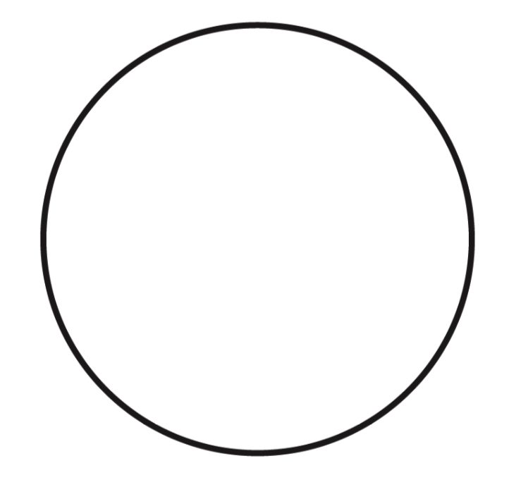
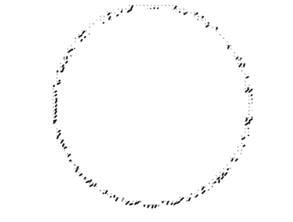
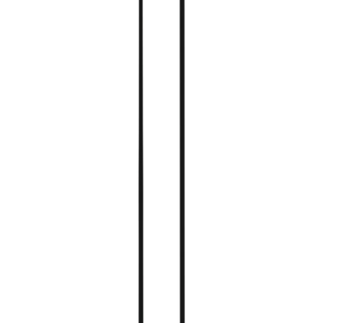
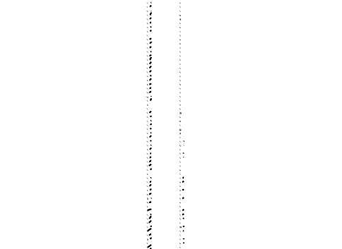
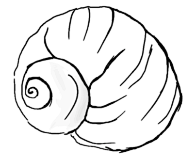
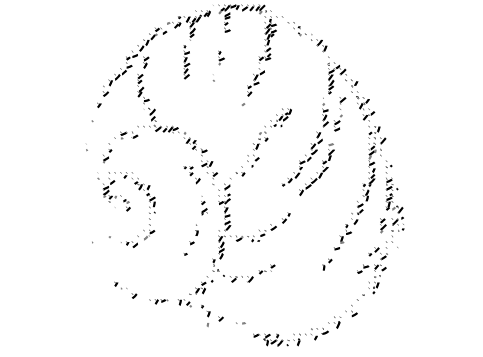
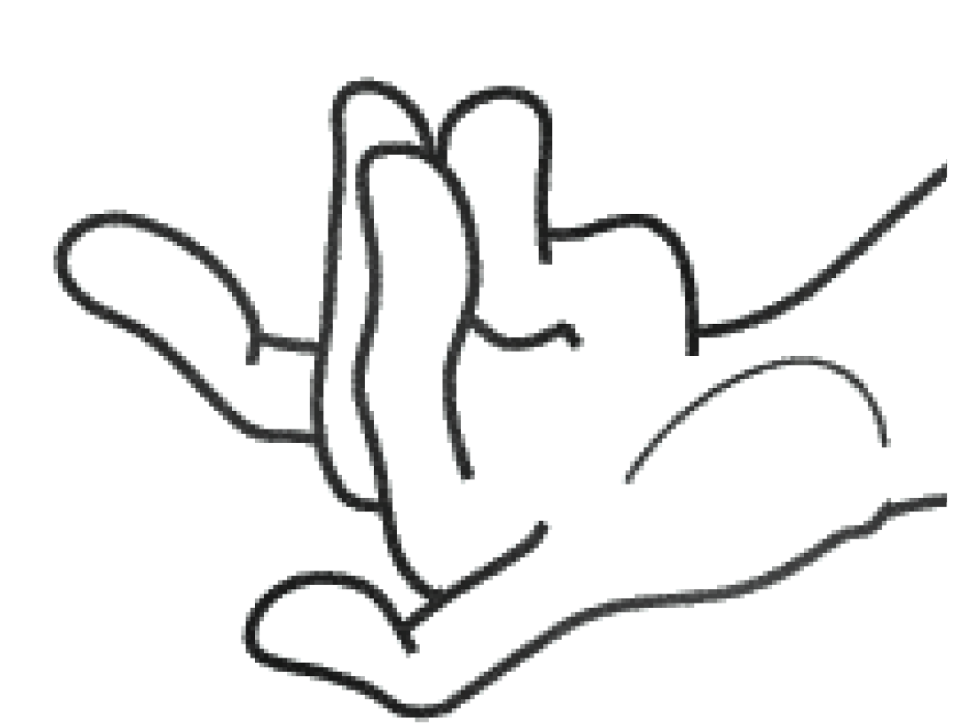
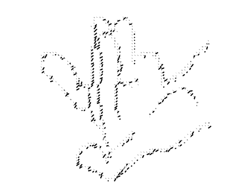
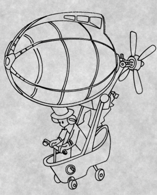
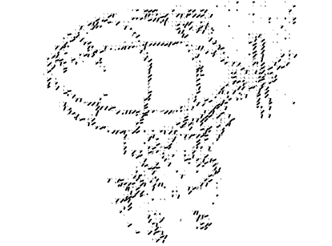
Though the curves mimic the structure of the original sketch, they are not always in the same direction as in the actual sketch. It seems like the curves assume this orientation to depict the thickness of the sketch lines.
Conclusion
Our initial plan was to utilize the code developed in the first week to create a differentiable vectorization. This approach would involve differentiating the functions we wrote to find the endpoints and intersections with respect to the coefficients of the bicubic curve. We would also use the tangents we calculated to determine the curve that best fits the original sketch.
Throughout the project, we worked with bicubic curves to ensure intersections and continuity of isolines between adjacent grid cells. However, we suspect that biquadratic curves might be sufficient for our needs and could significantly improve the implementation’s effectiveness. We are yet to confirm this and also explore whether an even lower degree might be feasible.
This project has opened up exciting avenues for future work and the potential to refine our methods further promises valuable contributions to the field. I am deeply grateful to Mikhail and Daniel for their guidance and support throughout this project.
References:
{1} Guillard, Benoit, et al. “MeshUDF: Fast and Differentiable Meshing of Unsigned Distance Field Networks”, ECCV 2022, https://doi.org/10.48550/arXiv.2111.14549
{2} Yan, Chuan, et al. “Deep Sketch Vectorization via Implicit Surface Extraction” SIGGRAPH 2024, https://doi.org/10.1145/3658197.
{3} Liu, Shichen, et al. “Soft Rasterizer: A Differentiable Renderer for Image-based 3D Reasoning” ICCV 2019, https://doi.org/10.48550/arXiv.1904.01786.
{4} “Bicubic Interpolation”. Wikipedia, https://en.wikipedia.org/wiki/Bicubic_interpolation.
{5} SciPy – fsolve (scipy.optimize.fsolve), https://docs.scipy.org/doc/scipy/reference/generated/scipy.optimize.fsolve.html