SGI Fellows: Harini Rammohan, Dianlun Luo, Idil Sulo
Project Mentor: Minghao Guo
SGI Volunteer: Shanthika Naik
Introduction:
TetSphere Splatting [Guo et al., 2024] is a cutting-edge technique for high-quality 3D shape reconstruction using tetrahedral meshes. This method stands out by delivering superior geometry without relying on neural networks or post-processing. Unlike traditional Eulerian methods, TetSphere Splatting excels in applications such as single-view 3D reconstruction and text-to-3D generation.
Our project aimed to enhance TetSphere Splatting through two key improvements:
- Geometry Optimization: We integrated subdivision and remeshing techniques to refine the geometry optimization process, enabling the capture of finer details and better tessellation.
- Adaptive TetSphere Modification: We developed adaptive mechanisms for splitting and merging tetrahedral spheres, enhancing flexibility and detail in the optimization process.
Setting up the Code Base:
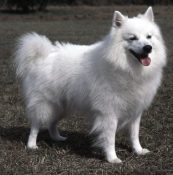
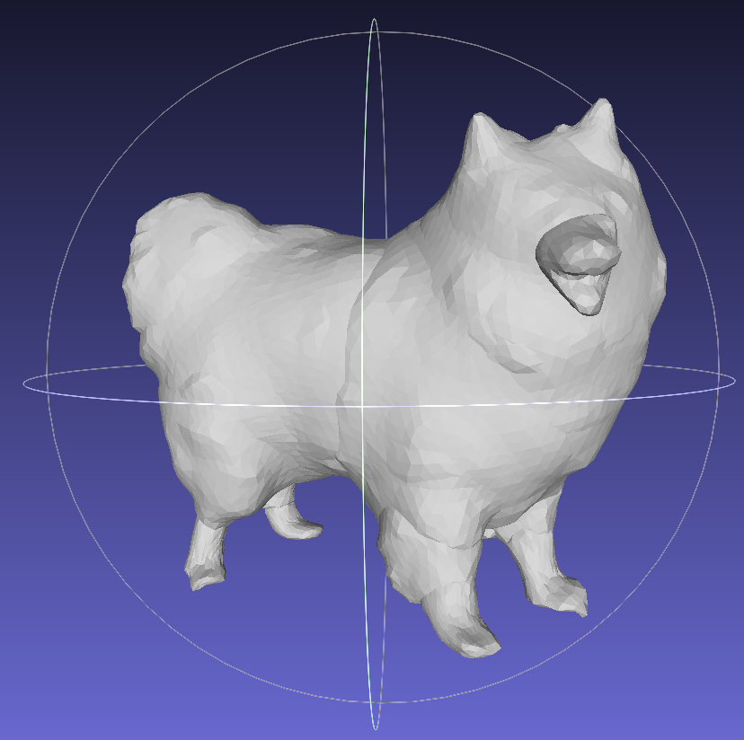
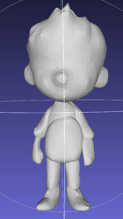
Our mentor, Minghao, facilitated the setup of the codebase in a cloud environment equipped with GPU support. Using a VSCode tunnel, we were able to work remotely and make modifications within the same environment. Following the instructions in the TetSphere Splatting GitHub README file, we successfully initialized the TetSpheres and executed the TetSphere Splatting process for our input images, including those of a white dog and a cartoon boy.

Geometry Optimization:
To improve the geometry optimization in TetSphere Splatting, we explored various algorithms for adaptive remeshing and subdivision. Initially, we considered parametrization-based remeshing using Centroidal Voronoi Tessellation (CVT) but opted for direct surface remeshing due to its efficiency and simplicity. For subdivision, we chose the Loop subdivision algorithm, as it is specifically designed for triangle meshes and better suited for our application compared to Catmull-Clark.
Implementing Loop Subdivision:
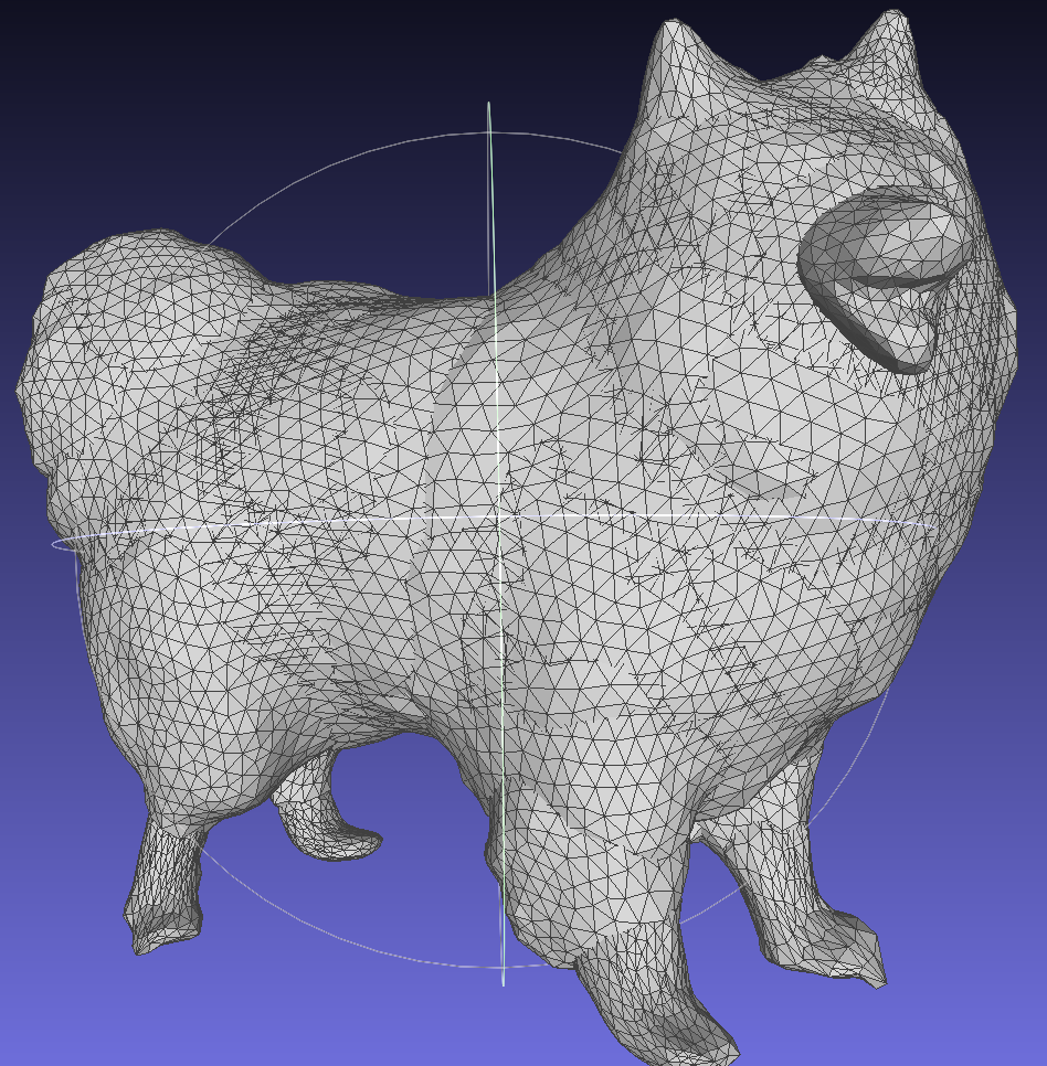
In the second week of the project, I worked on implementing the loop subdivision algorithm and incorporating it into the Geometry Optimization pipeline. Below is a detailed explanation of the algorithm and the method of implementation using the example of the example of the white dog mesh after TetSphere splatting.
1. Importing the required libraries, loading and initializing the mesh:
Instead of working throughout with numpy arrays, I chose to use defaultdict, a subclass of Python dictionaries to reduce the running time of the program. unique_edges defined below ensures that the list of edges doesn’t count each edge twice, once as (e1, e2) and once as (e2, e1).
import trimesh
import numpy as np
from collections import defaultdict

init_mesh = trimesh.load("./results/a_white_dog/final/final_surface_mesh.obj")
V = init_mesh.vertices
F = init_mesh.faces
E = init_mesh.edges

def unique_edges(edges):
    sorted_edges = np.sort(edges, axis=1)
    unique_edges = np.unique(sorted_edges, axis=0)
    return unique_edges
2. Edge-Face Adjacency Mapping
This maps edges to the faces they belong to, which will later help to identify boundary and interior edges.
def compute_edge_face_adjacency(faces):
    edge_face_map = defaultdict(list)
    for i, face in enumerate(faces):
        v0, v1, v2 = face
        edges = [(min(v0, v1), max(v0, v1)),
                 (min(v1, v2), max(v1, v2)),
                 (min(v2, v0), max(v2, v0))]
        for edge in edges:
            edge_face_map[edge].append(i)
    return edge_face_map
3. Computing New Vertices:
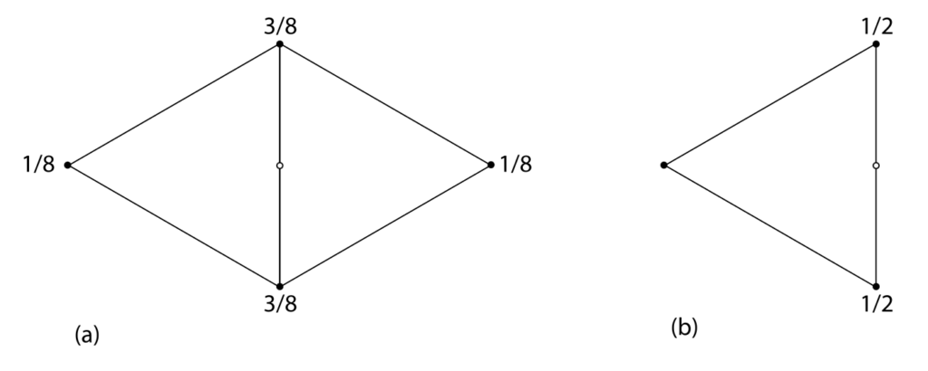
If an edge is a boundary edge (it belongs to only one face), then the new vertex is simply the midpoint of the two vertices at the ends of the edge. If not, the edge belongs to two faces and the new vertex is found to be a weighted average of the four vertices which make the two faces, with a weight of 3/8 for the vertices on the edge and 1/8 for the vertices not on the edge. The function also produces indices for the new vertices.
def compute_new_vertices(edge_face_map, vertices, faces):
    new_vertices = defaultdict(list)
    i = vertices.shape[0] - 1
    for edge, facess in edge_face_map.items():
        v0, v1 = edge
        if len(facess) == 1:  # Boundary edge
            i += 1
            new_vertices[edge].append(((vertices[v0] + vertices[v1]) / 2, i))
        elif len(facess) == 2:  # Internal edge
            i += 1
            adjacent_vertices = []
            for face_index in facess:
                face = faces[face_index]
                for vertex in face:
                    if vertex != v0 and vertex != v1:
                        adjacent_vertices.append(vertex)
            v2 = adjacent_vertices[0]
            v3 = adjacent_vertices[1]
            new_vertices[edge].append(((1 / 8) * (vertices[v2] + vertices[v3]) +
                                       (3 / 8) * (vertices[v0] + vertices[v1]), i))
    return new_vertices
4. Create a dictionary of updated vertices:
This generates updated vertices that include both old and newly created vertices.
def generate_updated_vertices(new_vertices, vertices, edges):
    updated_vertices = defaultdict(list)
    for i in range(vertices.shape[0]):
        vertex = vertices[i, :]
        updated_vertices[i].append(vertex)
    for i in range(edges.shape[0]):
        e1, e2 = edges[i, :]
        edge = (min(e1, e2), max(e1, e2))
        vertex, index = new_vertices[edge][0]
        updated_vertices[index].append(vertex)
    return updated_vertices
5. Construct New Faces:
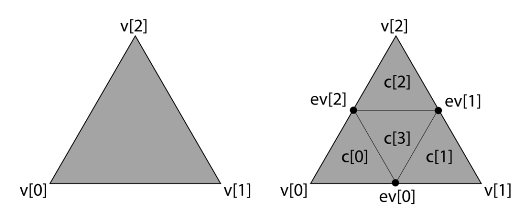
This constructs new faces using the updated vertices. Each old face is split into four new faces.
def create_new_faces(faces, new_vertices):
    new_faces = []
    for face in faces:
        v0, v1, v2 = face
        edge_0 = tuple(sorted((v0, v1)))
        edge_1 = tuple(sorted((v1, v2)))
        edge_2 = tuple(sorted((v2, v0)))

        e0 = new_vertices[edge_0][0][1]
        e1 = new_vertices[edge_1][0][1]
        e2 = new_vertices[edge_2][0][1]

        new_faces.append([v0, e0, e2])
        new_faces.append([v1, e1, e0])
        new_faces.append([v2, e2, e1])
        new_faces.append([e0, e1, e2])

    return np.array(new_faces)
6. Modifying Old Vertices Based on Adjacency:
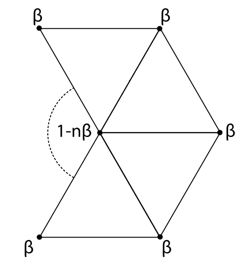
First, the function compute_vertex_adjacency finds the neighbors of each vertex. Then modify_vertices weights each of the neighbor vertices of each old vertex by a weight β (defined in the code below) and weights the old vertex by 1-nβ, where n is the degree of the old vertex. It does not change the new vertices.
def compute_vertex_adjacency(faces):
    vertex_adj_map = defaultdict(set)
    for face in faces:
        v0, v1, v2 = face
        vertex_adj_map[v0].add(v1)
        vertex_adj_map[v0].add(v2)
        vertex_adj_map[v1].add(v0)
        vertex_adj_map[v1].add(v2)
        vertex_adj_map[v2].add(v0)
        vertex_adj_map[v2].add(v1)
    return vertex_adj_map

def modify_vertices(vertices, updated_vertices, vertex_adj_map):
    modified_vertices = defaultdict(list)
    for i in range(len(updated_vertices)):
        if i in range(vertices.shape[0]):
            vertex = vertices[i,:]
            neighbors = vertex_adj_map[i]
            n = len(neighbors)
            beta = (5 / 8 - (3 / 8 + 1 / 4 * np.cos(2 * np.pi / n)) ** 2)/n
            weight_v = 1 - beta * n
            modified_vertex = weight_v * vertex
            for neighbor in neighbors:
                neighbor_point = updated_vertices[neighbor][0]
                modified_vertex += beta * neighbor_point
            modified_vertices[i].append(modified_vertex)
        else:
            modified_vertices[i].append(updated_vertices[i][0])
    return modified_vertices
7. Generating the Final Subdivided Mesh:
Now, all that is left is to collect the modified vertices and faces as numpy arrays and create the final subdivided mesh. The function loop_subdivision_iter simply applies the loop subdivision iteratively ‘n’ times, further refining the loop each time.
def create_vertices_array(modified_vertices):
    vertices_list = [modified_vertices[i][0] for i in range(len(modified_vertices))]
    return np.array(vertices_list)

def loop_subdivision(vertices, faces, edges):
    edges = unique_edges(edges)
    edge_face_map = compute_edge_face_adjacency(faces)
    new_vertices = compute_new_vertices(edge_face_map, vertices, faces)
    updated_vertices = generate_updated_vertices(new_vertices, vertices, edges)
    new_faces = create_new_faces(faces, new_vertices)
    vertex_adj_map = compute_vertex_adjacency(new_faces)
    modified_vertices = modify_vertices(vertices, updated_vertices, vertex_adj_map)
    vertices_array = create_vertices_array(modified_vertices)
    return vertices_array, new_faces

def loop_subdivision_iter(vertices, faces, n):
    def unique_edges(faces):
            edges = np.vstack([
            np.column_stack((faces[:, 0], faces[:, 1])),
            np.column_stack((faces[:, 1], faces[:, 2])),
            np.column_stack((faces[:, 2], faces[:, 0]))
                ])
            sorted_edges = np.sort(edges, axis=1)
            unique_edges = np.unique(sorted_edges, axis=0)
            return unique_edges
    if n == 0:
        edges = unique_edges(faces)
        return loop_subdivision(V, F, E)
    else:
        edges = unique_edges(faces)
        vertices, faces = loop_subdivision(vertices, faces, edges)
        output = loop_subdivision_iter(vertices, faces, n-1)
        return output

new_V, new_F = loop_subdivision_iter(V, F, 1)
subdivided_mesh = trimesh.Trimesh(vertices=new_V, faces=new_F)
subdivided_mesh.export("./a_white_dog_subdivided.obj")
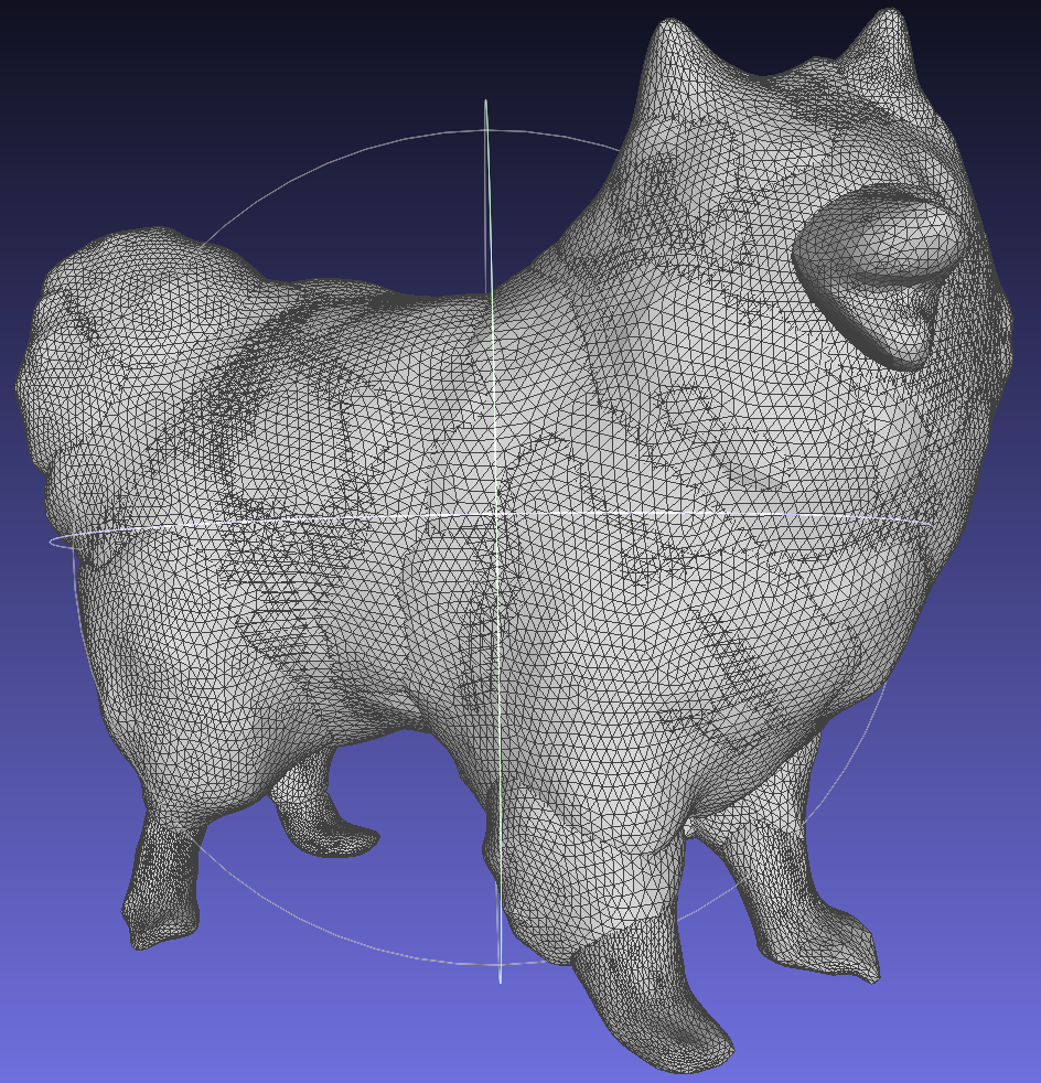
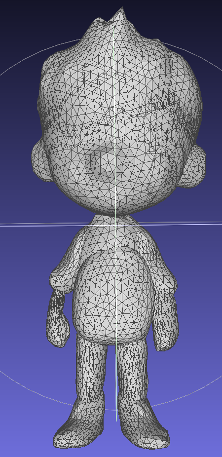
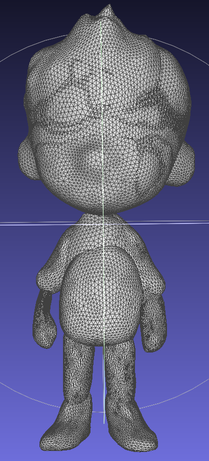
Results:
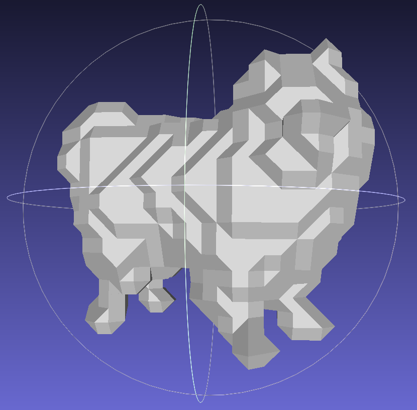
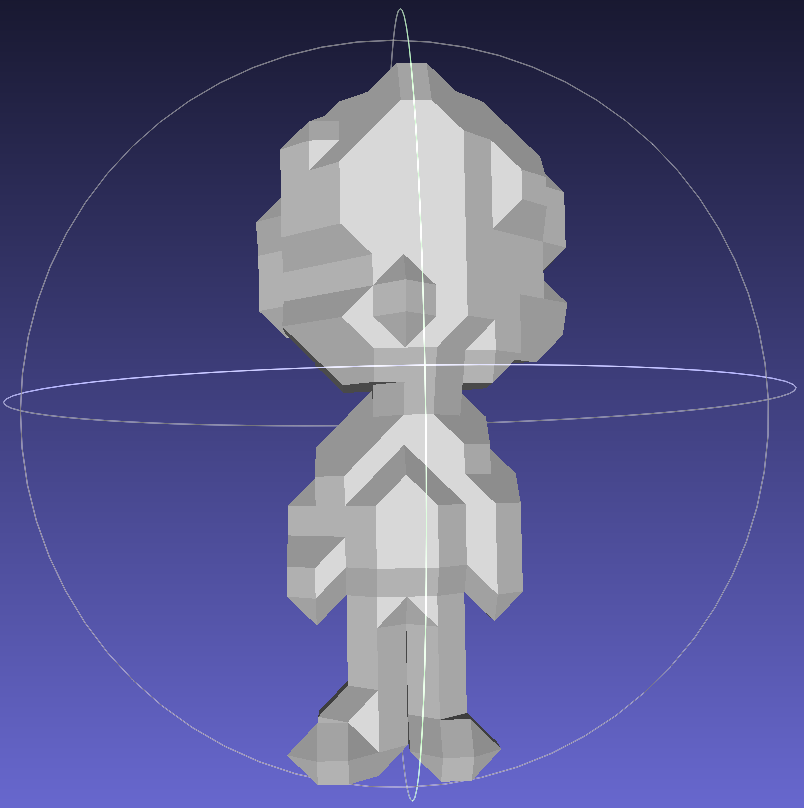
I used the above code to obtain the subdivided meshes for four input meshes – a white dog, a cartoon boy, a camel, and a horse. The results for each of these are displayed below.
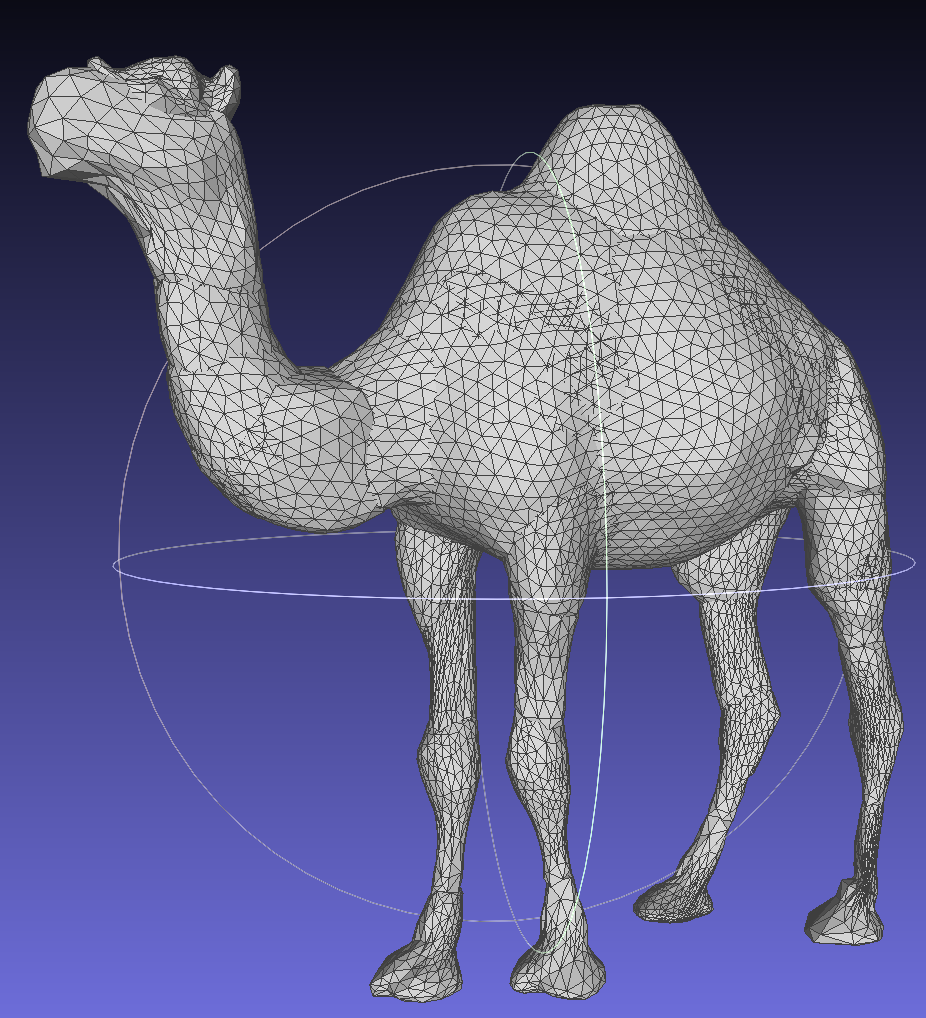
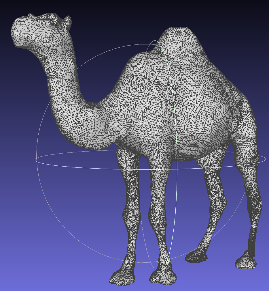
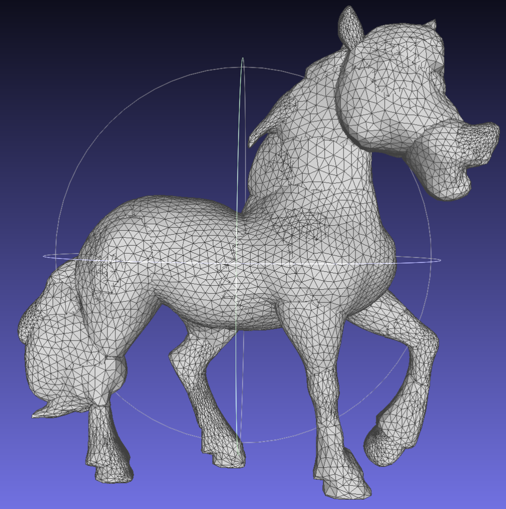
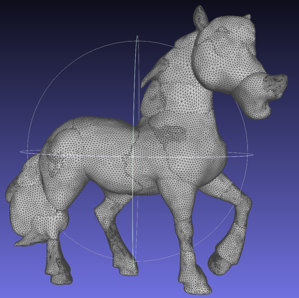
Conclusion:
The project successfully enhanced the TetSphere Splatting method through geometry optimization and adaptive TetSphere modification. The implementation of Loop subdivision refined mesh detail and smoothness, as evidenced by the improved results for the test meshes. The adaptive mechanisms introduced greater flexibility, contributing to more precise and detailed 3D reconstructions.
Through this project I learned a lot about TetSphere Splatting, Geometry Optimization and Loop Subdivion. I am very grateful to Minghao and Shanthika who supported and guided us in our progress.
References:
{1} Guo, Minghao, et al. “TetSphere Splatting: Representing High-Quality Geometry with Lagrangian Volumetric Meshes”, https://doi.org/10.48550/arXiv.2405.20283
{2} Kerbl, Bernhard, et al. “3D Gaussian Splatting
for Real-Time Radiance Field Rendering” SIGGRAPH 2023, https://doi.org/10.48550/arXiv.2308.04079.
{3} “Remeshing I”, https://graphics.stanford.edu/courses/cs468-12-spring/LectureSlides/13_Remeshing1.pdf
{4} “Subdivision”, https://www.cs.cmu.edu/afs/cs/academic/class/15462-s14/www/lec_slides/Subdivision.pdf
{5} Pharr, Matt, et al. “Physically Based Rendering: From Theory To Implementation – 3.8 Subdivision Surfaces”, https://www.pbr-book.org/3ed-2018/Shapes/Subdivision_Surfaces.