Primary mentor: Minghao Guo
Volunteer assistant: Shanthika Naik
Student: Dianlun (Jennifer) Luo
1. Introduction
TetSphere Splatting, introduced by Guo et al. (2024), is a cutting-edge method for reconstructing 3D shapes with high-quality geometry. It employs an explicit, Lagrangian geometry representation to efficiently create high-quality meshes. Unlike conventional object reconstruction techniques, which typically use Eulerian representations and face challenges with high computational demands and suboptimal mesh quality, TetSphere Splatting leverages tetrahedral meshes, providing superior results without the need for neural networks or post-processing. This method is robust and versatile, making it suitable for a wide range of applications, including single-view 3D reconstruction and image-/text-to-3D content generation.
The primary objective of this project was to explore volumetric geometry reconstruction through the implementation of two key enhancements:
- Geometry Optimization via Subdivision/Remeshing: This involved integrating subdivision and remeshing techniques to refine the geometry optimization process in TetSphere Splatting, allowing for the capture of finer details and improving overall tessellation quality.
- Adaptive TetSphere Modification: Mechanisms were developed to adaptively split and merge tetrahedral spheres during the optimization phase, enhancing the flexibility of the method and improving geometric detail capture.
In this project, I implemented Adaptive Isotropic Remeshing from scratch. The algorithm was tested on two models:
- final_surface_mesh.obj generated by TetSphere Splatting in the TetSphere Splatting codebase.
- The Stanford Bunny mesh (bun_zipper_res2.ply).
2. Adaptive Isotropic Remeshing Algorithm
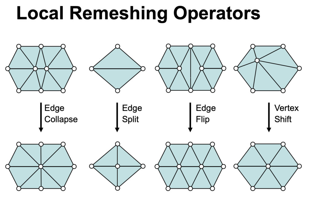
The remeshing procedure can be broken down into four major steps:
- Split all edges at their midpoint that are longer than \( \frac{4}{3} l \), where \( l \) is the local sizing field.
- Collapse all edges shorter than \( \frac{4}{5} l \) into their midpoint.
- Flip edges in order to minimize the deviation from the ideal vertex valence of 6 (or 4 on boundaries).
- Relocate vertices on the surface by applying tangential smoothing.
2.1 Adaptive Sizing Field
Instead of using a uniform target edge length, an adaptive sizing field was computed using the trimesh package. The constant target edge length \( L \) was replaced by an adaptive sizing field \( L(x) \), which is intuitive to control, simple to implement, and efficient to compute.
Splitting edges based on their length and the angle of their endpoint normals can lead to anisotropically stretched triangles, requiring an additional threshold parameter to control the allowed deviation of endpoint normals. The remeshing approach is based on a single, highly intuitive parameter: the approximation tolerance \( \epsilon \). This parameter controls the maximum allowed geometric deviation between the triangle mesh and the underlying smooth surface geometry.
The method first computes the curvature field of the input mesh and then derives the optimal local edge lengths (the sizing field \( L(x) \)) from the maximum curvature and the approximation tolerance. The process is as follows:
Algorithm: Compute Adaptive Sizing Field

Input: Mesh M, Points P, Parameter ε
Output: Sizing Field Values S

Step 1: Compute Mean Curvature
    H ← discrete_mean_curvature_measure(M, P, radius = 1.0)

Step 2: Compute Gaussian Curvature
    K ← discrete_gaussian_curvature_measure(M, P, radius = 1.0)

Step 3: Compute Maximum Curvature
    C_max ← |H| + sqrt(|H² - K|)

Step 4: Ensure Minimum Curvature Threshold
    C_max ← max(C_max, 1e-6)

Step 5: Compute Sizing Field Values
    S ← sqrt(max((6ε / C_max) - 3ε², 0))

Step 6: Return Sizing Field Values
    Return S
2.2 Edge Splitting
Edge splitting is a process where edges that exceed a certain length threshold are split at their midpoint. This step helps maintain consistent element sizes across the mesh and prevent the occurrence of overly stretched or irregular elements. By splitting longer edges, we can achieve better mesh quality, improve computational efficiency, and optimize the mesh for various applications.
Algorithm: Split Edges of a Mesh

Input: Mesh M, Parameter ε
Output: Modified Mesh with Split Edges

Step 1: Initialize new vertex and face lists
    new_vertices ← M.vertices
    new_faces ← M.faces

Step 2: Iterate over each edge in the mesh
    For each edge e = (v₀, v₁) in M.edges:
        - Compute edge length: l_edge ← ||M.vertices[v₀] - M.vertices[v₁]||
        - Compute sizing field for edge vertices: sizing_values ← sizing_field(M, [v₀, v₁], ε)
        - Calculate target length: l_target ← (sizing_values[0] + sizing_values[1]) / 2

        If l_edge > (4/3) * l_target:
            Step 3: Split the edge
                - Compute midpoint: midpoint ← (M.vertices[v₀] + M.vertices[v₁]) / 2
                - Add the new vertex to new_vertices
                - Find adjacent faces containing edge (v₀, v₁)
                - For each adjacent face f = (v₀, v₁, v₂):
                    - Remove face f from new_faces
                    - Add new faces [v₀, new_vertex, v₂] and [v₁, new_vertex, v₂] to new_faces

Step 4: Create and return new mesh
    Return M ← trimesh.Trimesh(vertices=new_vertices, faces=new_faces)
2.3 Edge Collapse
Edge collapse simplifies the mesh by merging the vertices of short edges. This step is particularly useful for eliminating unnecessary small elements that may introduce inefficiencies in the mesh. By collapsing short edges, the mesh is coarsened in areas where high detail is not needed.
Algorithm: Collapse Edges of a Mesh

Input: Mesh M, Parameter ε
Output: Modified Mesh with Collapsed Edges

Step 1: Initialize face list and sets
    new_faces ← M.faces
    vertices_to_remove ← []
    collapsed_vertices ← {}

Step 2: Iterate over each edge in the mesh
    For each edge e = (v₀, v₁) in M.edges:
        - Compute edge length: l_edge ← ||M.vertices[v₀] - M.vertices[v₁]||
        - Compute sizing field for edge vertices: sizing_values ← sizing_field(M, [v₀, v₁], ε)
        - Calculate target length: l_target ← (sizing_values[0] + sizing_values[1]) / 2

        If l_edge < (4/5) * l_target and v₀, v₁ not in collapsed_vertices:
            Step 3: Collapse the edge
                - Compute midpoint: midpoint ← (M.vertices[v₀] + M.vertices[v₁]) / 2
                - Set M.vertices[v₀] ← midpoint
                - Mark v₁ for removal: vertices_to_remove ← vertices_to_remove ∪ {v₁}
                - Mark v₀, v₁ as collapsed: collapsed_vertices ← collapsed_vertices ∪ {v₀, v₁}

                Find adjacent faces containing v₁ but not v₀:
                For each adjacent face f = (v₁, v₂, v₃):
                    - Remove face f from new_faces
                    - Add new face [v₀, v₂, v₃] to new_faces
                    - Mark v₂, v₃ as collapsed

Step 4: Update the mesh
    - Create index_map to remap vertex indices for remaining vertices
    - Remove vertices in vertices_to_remove from M.vertices
    - Remap the faces in new_faces based on index_map

Step 5: Create and return new mesh
    Return M ← trimesh.Trimesh(vertices=new_vertices, faces=new_faces)
2.4 Edge Flipping
Edge flipping is performed when it reduces the squared difference between the actual valence of the four vertices in the two adjacent triangles and their optimal values. For interior vertices, the ideal valence is 6, while for boundary vertices, it is 4.
To preserve key features of the mesh, sharp edges and material boundaries should not be flipped.
Algorithm: Check Edge Flip Condition

Input: Vertices V, Edges E, Faces F, Edge e = (v₁, v₂)
Output: Flip Condition, New Vertices v₃, v₄, Adjacent Faces f₁, f₂

Step 1: Find adjacent faces of edge e
    adjacent_faces ← [f ∈ F : v₁ ∈ f and v₂ ∈ f]

    If len(adjacent_faces) ≠ 2:
        Return False, None, None, None, None

Step 2: Identify third vertices of adjacent faces
    f₁, f₂ ← adjacent_faces
    v₃ ← [v ∈ f₁ : v ≠ v₁ and v ≠ v₂]
    v₄ ← [v ∈ f₂ : v ≠ v₁ and v ≠ v₂]

    If len(v₃) ≠ 1 or len(v₄) ≠ 1 or v₃[0] = v₄[0]:
        Return False, None, None, None, None

Step 3: Check edge conditions
    v₃, v₄ ← v₃[0], v₄[0]

    If [v₃, v₄] ∈ E:
        Return False, None, None, None, None

Step 4: Check normal vector alignment
    Compute normal₁ ← normal(f₁), normal₂ ← normal(f₂)
    Normalize both normal₁ and normal₂
    Compute dot product dot_product ← dot(normal₁, normal₂)

    If dot_product < 0.9:
        Return False, None, None, None, None

Step 5: Compute valence difference before and after edge flip
    valence ← compute_valence(V, E)
    Compute valence difference before and after the flip

Return difference_after < difference_before, v₃, v₄, f₁, f₂
Algorithm: Flip Edge of a Mesh
Input: Mesh M, Edge e = (v₁, v₂)
Output: Modified Mesh M
Step 1: Check if edge flip condition is satisfied
condition, v₃, v₄, f₁, f₂ ← flip_edge_condition(M.vertices, M.edges_unique, M.faces, e)
If condition = False:
Return M
Step 2: Update the faces
Remove f₁ and f₂ from the mesh faces
Add new faces [v₁, v₃, v₄] and [v₂, v₃, v₄] to the mesh
Step 3: Create and return the updated mesh
Return new_mesh ← trimesh.Trimesh(vertices=M.vertices, faces=new_faces)2.5 Tangential Relaxation
Tangential smoothing relocates vertices to create a smoother surface without significantly altering the mesh geometry. The process averages the positions of the neighboring vertices, constrained to the surface, which maintains the mesh’s adherence to the original geometry while improving its smoothness.
Algorithm: Tangential Relaxation

Input: Mesh M, Sizing Field L
Output: Relaxed Mesh

Step 1: Initialize variables
    vertices ← M.vertices
    faces ← M.faces
    relaxed_vertices ← zeros_like(vertices)

Step 2: For each vertex i in vertices:
    Find incident faces for vertex i
        incident_faces ← where(faces == i)
        weighted_barycenter_sum ← zeros(3)
        weight_sum ← 0

    Step 3: For each face f in incident_faces:
        Compute barycenter and area
            face_vertices ← faces[f]
            triangle_vertices ← vertices[face_vertices]
            barycenter ← mean(triangle_vertices)

            v₀, v₁, v₂ ← triangle_vertices
            area ← ||cross(v₁ - v₀, v₂ - v₀)|| / 2

        Step 4: Compute weight based on sizing field
            sizing_at_barycenter ← mean([L[v] for v in face_vertices])
            weight ← area × sizing_at_barycenter

        Step 5: Accumulate weighted barycenter sum
            weighted_barycenter_sum ← weighted_barycenter_sum + weight × barycenter
            weight_sum ← weight_sum + weight

    Step 6: Compute relaxed vertex position
        relaxed_vertices[i] ← weighted_barycenter_sum / weight_sum if weight_sum ≠ 0 else vertices[i]

Step 7: Create and return relaxed mesh
    Return relaxed_mesh ← trimesh.Trimesh(vertices=relaxed_vertices, faces=faces)
2.6 Adaptive Remeshing
The adaptive remeshing algorithm iterates through the above steps to refine the mesh over multiple iterations.
Algorithm: Adaptive Remeshing

Input: Mesh M, Parameter ε, Number of Iterations: iteration
Output: Remeshed and Smoothed Mesh

For i = 1 to iteration:

    Step 1: Split edges
        M ← split_edges(M, ε)

    Step 2: Collapse edges
        M ← collapse_edges(M, ε)

    Step 3: Flip edges
        For each edge e in M.edges_unique:
            M ← flip_edge(M, e)

    Step 4: Tangential relaxation
        Recalculate sizing values based on the updated mesh
        sizing_values ← sizing_field(M, M.vertices, ε)
        M ← tangential_relaxation(M, sizing_values)

Return M
3. Results
3.1 final_surface_mesh.obj
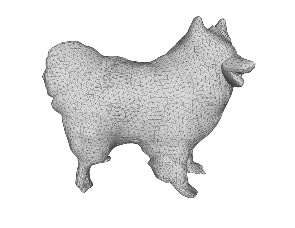
The TetSphere Splatting output (final_surface_mesh.obj) and its corresponding remeshed version (dog_remeshed_iter1.obj) were evaluated to assess the effectiveness of the remeshing algorithm.
- final_surface_mesh.obj:
- Vertices: 16,675
- Faces: 33,266
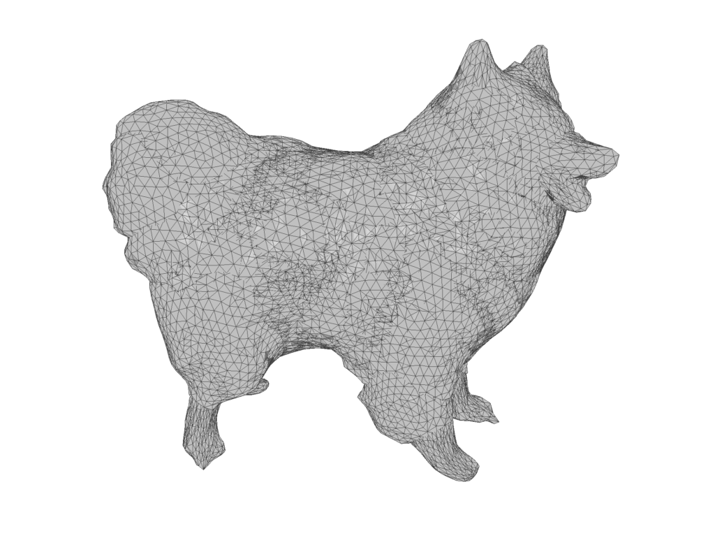
- dog_remeshed_iter1.obj:
- Vertices: 26,603
- Faces: 53,122
Comparison:
The remeshing process results in a significant increase in both vertices and faces, which produces a more refined and detailed mesh. This is clear in the comparison image below. The dog_remeshed_iter1.obj (right) shows a denser mesh structure compared to the final_surface_mesh.obj (left). The Adaptive Isotropic Remeshing algorithm enhances resolution and captures finer geometric details.
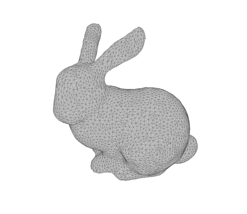
3.2 bun_zipper_res2.ply
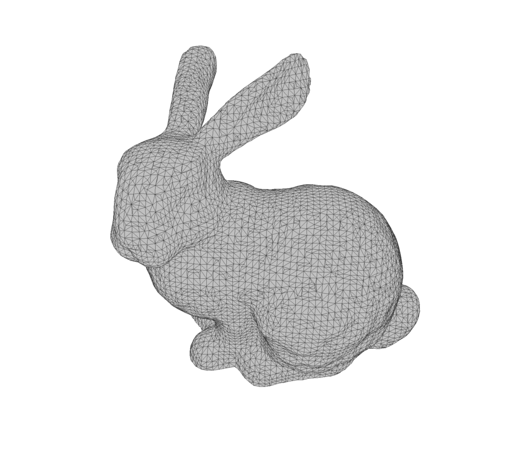
The Stanford Bunny mesh (bun_zipper_res2.ply) was similarly processed through multiple iterations of remeshing to evaluate the progressive refinement of the mesh.
- bun_zipper_res2.ply:
- Vertices: 8,171
- Faces: 16,301
- bunny_remeshed_iter1.obj:
- Vertices: 6,476
- Faces: 12,962
- bunny_remeshed_iter2.obj:
- Vertices: 5,196
- Faces: 10,381
- bunny_remeshed_iter3.obj:
- Vertices: 4,159
- Faces: 8,300
Comparison:
The progressive reduction in vertices and faces over the iterations demonstrates the remeshing algorithm’s ability to simplify the mesh while retaining the overall geometry. The remeshed iterations display a higher number of equilateral triangles, which creates a more uniform and well-proportioned mesh. This improvement is obvious when comparing the final iteration (bunny_remeshed_iter3.obj) with the original model (bun_zipper_res2.ply). The triangles become more equilateral and evenly distributed, resulting in a smoother and more consistent surface.


4. Performance Analysis
The current implementation of the remeshing algorithm was developed in Python, utilizing the trimesh library. While Python is easy to use, performance limitations may arise when handling large-scale meshes or real-time rendering.
A potential solution to improve performance is to transition the core remeshing algorithms to C++.
Benefits of Using C++:
- Speed: C++ allows for significantly faster execution times due to its lower-level memory management and optimization capabilities.
- Parallelization: Advanced threading and parallel computing techniques in C++ can accelerate the remeshing process.
- Memory Efficiency: C++ provides better control over memory allocation, which is crucial when working with large datasets.
5. References
M. Botsch and L. Kobbelt, “A remeshing approach to multiresolution modeling,” Proceedings of the 2004 Eurographics/ACM SIGGRAPH Symposium on Geometry Processing, Nice, France, 2004, pp. 185–192. doi: 10.1145/1057432.1057457.
M. Dunyach, D. Vanderhaeghe, L. Barthe, and M. Botsch, “Adaptive remeshing for real-time mesh deformation,” in Eurographics 2013 – Short Papers, M.-A. Otaduy and O. Sorkine, Eds. The Eurographics Association, 2013, pp. 29–32. doi: 10.2312/conf/EG2013/short/029-032.
“Remeshing,” Lecture Slides for CS468, Stanford University, 2012. [Online]. Available: https://graphics.stanford.edu/courses/cs468-12-spring/LectureSlides/13_Remeshing1.pdf. [Accessed: Sep. 12, 2024].
M. Guo, B. Wang, K. He, and W. Matusik, “TetSphere Splatting: Representing high-quality geometry with Lagrangian volumetric meshes,” arXiv, 2024. [Online]. Available: https://arxiv.org/abs/2405.20283. [Accessed: Sep. 12, 2024].
B. Kerbl, G. Kopanas, T. Leimkuehler, and G. Drettakis, “3D Gaussian splatting for real-time radiance field rendering,” ACM Trans. Graph., vol. 42, no. 4, Art. no. 139, Jul. 2023. doi: 10.1145/3592433.