Author: Krishna Chebolu
Teammates: Bethlehem Tassew and Kimberly Herrera
Mentor: Dr. Ankita Shukla
Introduction
For the past two weeks, our project team mentored by Dr. Ankita Shukla set out to understand the inner workings of OpenAI’s CLIP model. Specifically, we were interested in gaining a mathematical understanding of feature spaces’ geometric and topological properties.
OpenAI’s CLIP (Contrastive Language-Image Pre-Training) is a versatile and powerful model designed to understand and generate text and images. CLIP is trained to connect text and images by learning from a large dataset of images paired with their corresponding textual descriptions. The model is trained using a contrastive learning approach, where it learns to predict which text snippet is associated with which image from a set of possible pairs. This allows CLIP to understand the relationship between textual and visual information.
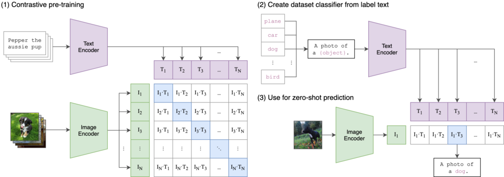
CLIP uses two separate encoders: a text encoder (based on the Transformer architecture) and an image encoder (based on a convolutional neural network or a vision transformer). Both encoders produce embeddings in a shared latent space (also called a feature space). By aligning text and image embeddings in the same space, CLIP can perform tasks that require cross-modal understanding, such as image captioning, image classification with natural language labels, and more.
CLIP is trained on a vast dataset containing 400 million image-text pairs collected online. This extensive training data allows it to generalize across various domains and tasks. One of CLIP’s standout features is its ability to perform zero-shot learning. It can handle new tasks without requiring task-specific training data, simply by understanding the task description in natural language. More information can be found in OpenAI’s paper.
In our attempts to understand the inner workings of the feature spaces, we employed tools from UMAP, persistence homology, subspace angles, cosine similarity matrices, and Wasserstein distances.
Our Study – Methodology and Results
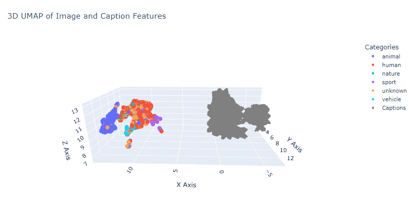
All of our teammates started with datasets that contained image-caption pairs. We classified images into various categories using their captions and embedded them using CLIP. Then we used UMAP or t-SNE plots to visualize their characteristics.
After this preliminary visualization, we desire to delve deeper. We introduced noise, a Gaussian blur, to our images to test CLIP’s robustness. We added the noise in increments (for example mean = 0, standard deviation = {1,2,3,4,5}) and encoded them as we did the original image-caption pairs. We then made persistence diagrams using ripser. We also followed the same procedure within the various categories to understand how noise impacts not only the overall space but also their respective subspaces. These diagrams for the five categories from the Flickr 8k dataset can be found in this Google Colab notebook.
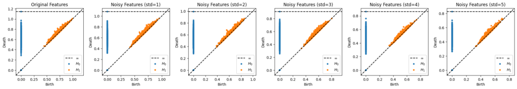
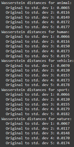
Visually, you can observe that there is no significant difference, which attests to CLIP’s robustness. However, visual assurance is not enough. Thus, we used Scipy’s Wasserstein’s distance calculation to note how different each persistence diagram is from the other. Continuing the same Flickr 8k dataset, for each category, we obtain the values shown in Figure 4.
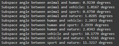
Another question to understand is how similar are each of the categories to one another. This question can be answered by calculating the subspace angles. After embedding, each category can be seen as occupying a space that can often be far away from another category’s space– we want to quantify how far away, so we use subspace angles. Results for the Flickr 8k dataset example are shown in Figure 5.
Conclusion
At the start, our team members were novices in the CLIP model, but we concluded as lesser novices. Through the two weeks, Dr. Shukla supported us and enabled us to understand the inner workings of the CLIP model. It is certainly thrilling to observe how AI around us is constantly evolving, but at the heart of it is mathematics governing the change. We are excited to possibly explore further and perform more analyses.