Categories
Research

A Study on Surface Reconstruction from Signed Distance Data Part 2: Error Methods

Primary mentors:  Silvia Sellán, University of Toronto and Oded Stein, University of Southern California

Volunteer assistant:  Andrew Rodriguez

Fellows: Johan Azambou, Megan Grosse, Eleanor Wiesler, Anthony Hong, Artur RB Boyago, Sara Samy

After talking about what are some of the ways to reconstruct sdfs (see part one), we now study the question of how to evaluate their performance. Two classes of error function are considered, the first more inherent to our sdf context, and the second more general in all situations. We will first show results by our old friends, Chamfer distance, Hausdorff distance, and area method (see here for example), and then introduce the inherent one.

Hausdorff and Chamfer Distance

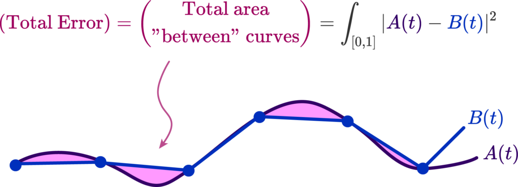
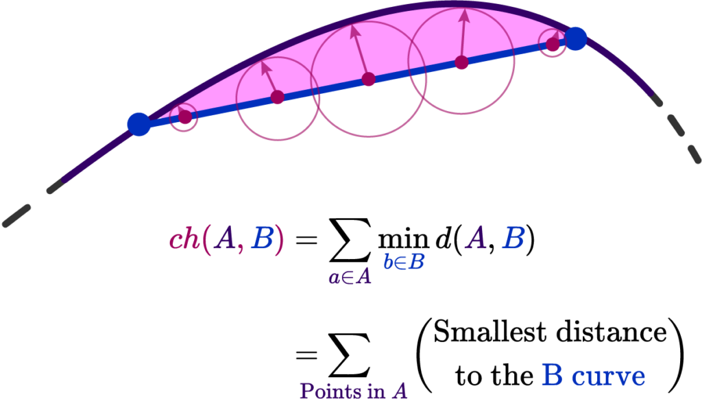
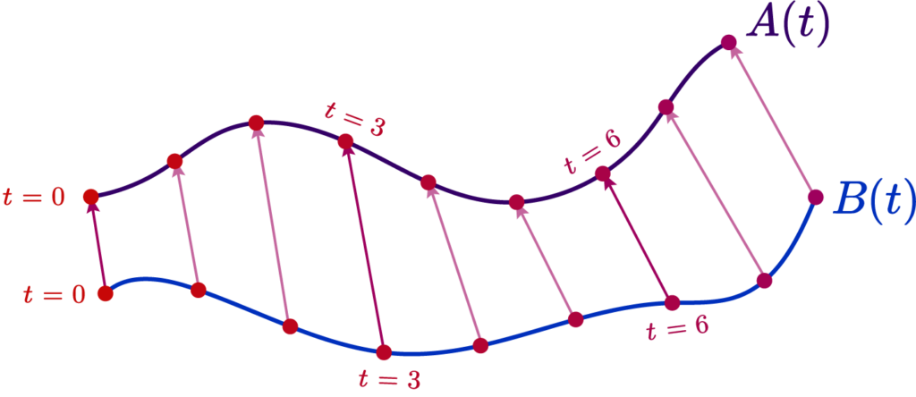
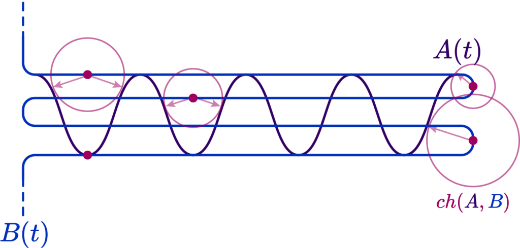
The Chamfer distance provides an average-case measure of the dissimilarity between two shapes. It calculates the sum of the distances from each point in one set to the nearest point in the other set. This measure is particularly useful when the goal is to capture the overall discrepancy between two shapes while being less sensitive to outliers. The Chamfer distance is defined as:
$$
d_{\mathrm{Chamfer }}(X, Y):=\sum_{x \in X} d(x, Y)=\sum_{x \in X} \inf _{y \in Y} d(x, y)
$$

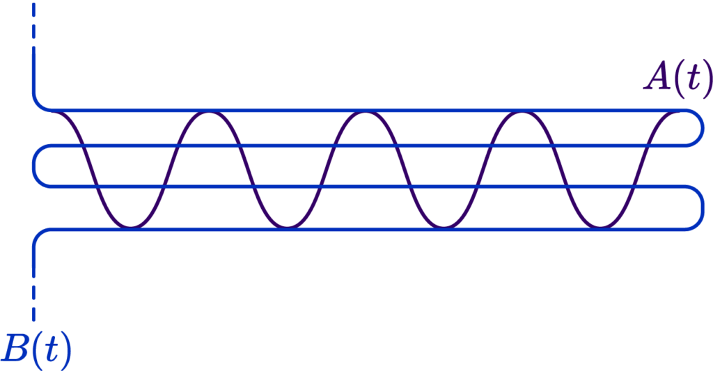
The Bi-Chamfer distance is an extension that considers the average of the Chamfer distance computed in both directions (from \(X\) to \(Y\) and from \(Y\) to \(X\) ). This bidirectional measure provides a more balanced assessment of the dissimilarity between the shapes:
$$
d_{\mathrm{B} \mathrm{-Chamfer }}(X, Y):=\frac{1}{2}\left(\sum_{x \in X} \inf {y \in Y} d(x, y)+\sum{y \in Y} \inf _{x \in X} d(x, y)\right)
$$

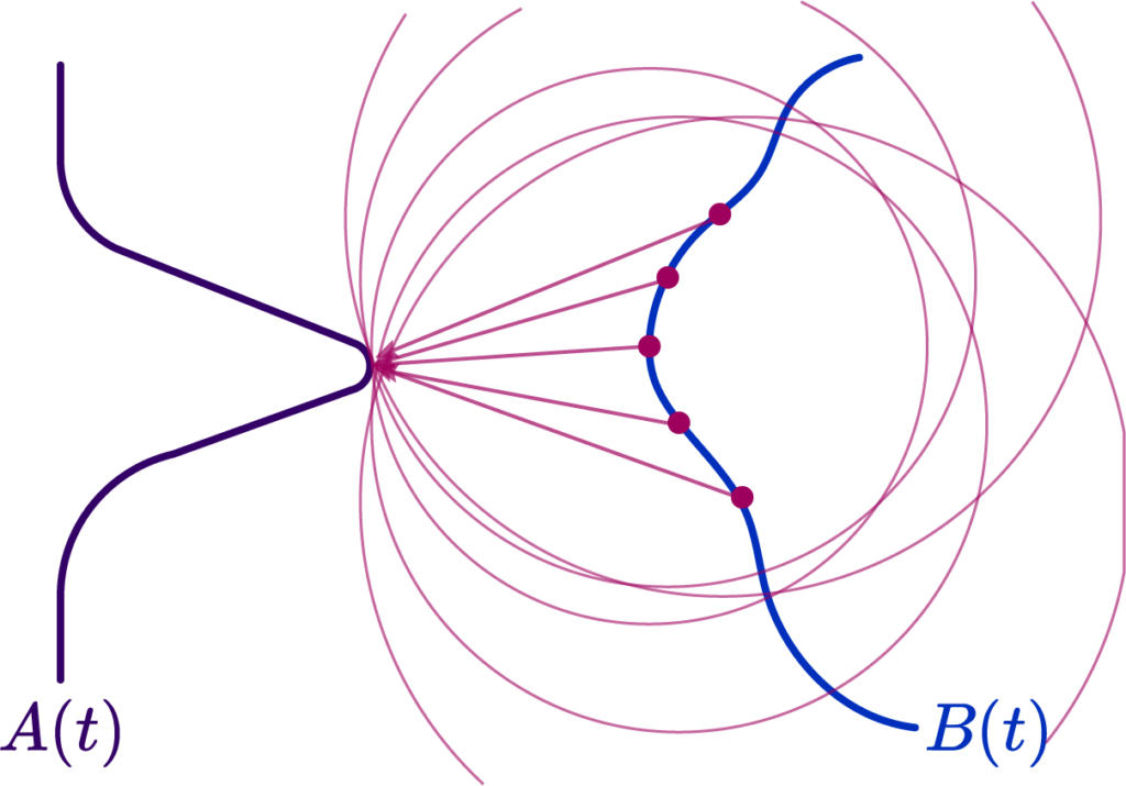
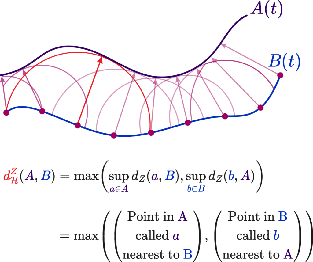
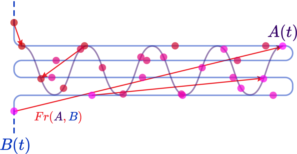
The Hausdorff distance, on the other hand, measures the worst-case scenario between two shapes. It is defined as the maximum distance from a point in one set to the closest point in the other set. This distance is particularly stringent because it reflects the largest deviation between the shapes, making it highly sensitive to outliers.

The formula for Hausdorff distance is:
$$
d_{\mathrm{H}}^Z(X, Y):=\max \left(\sup {x \in X} d_Z(x, Y), \sup {y \in Y} d_Z(y, X)\right)
$$

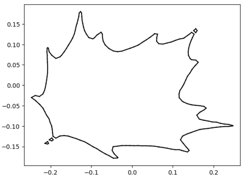
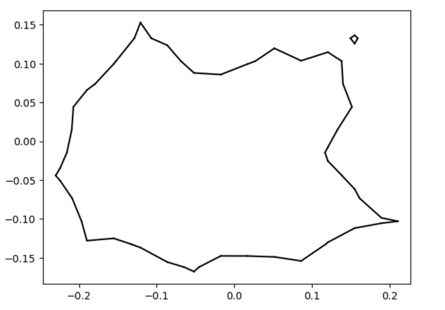
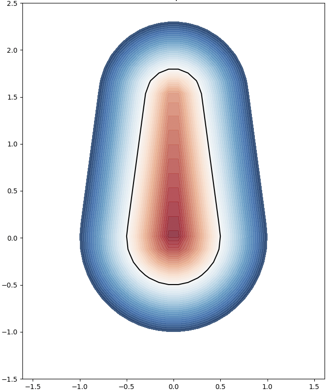
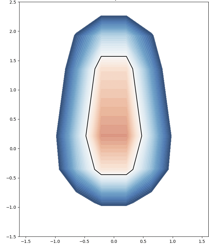
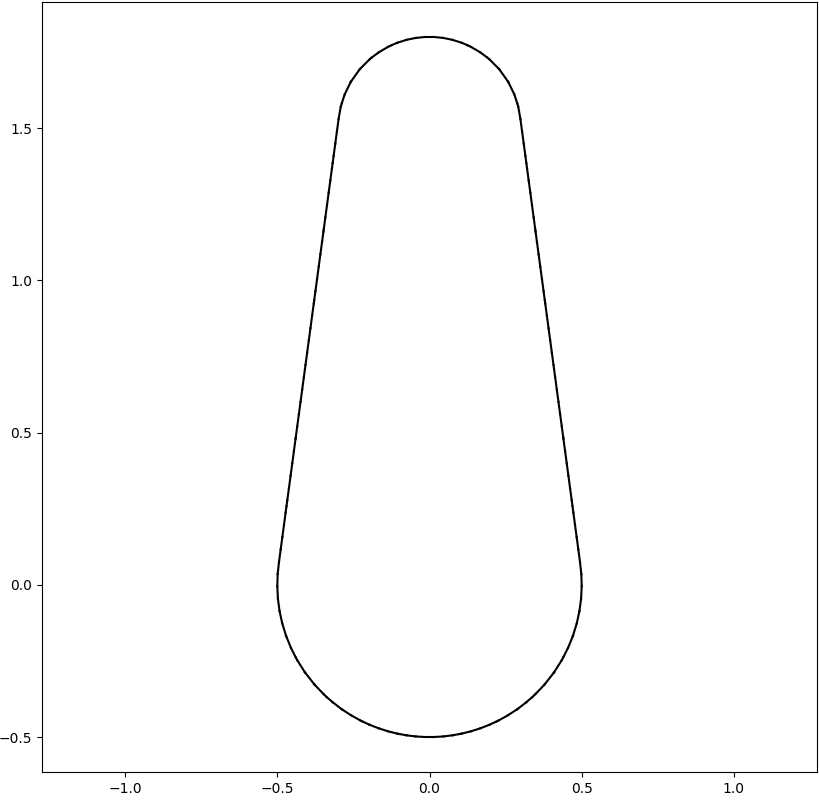
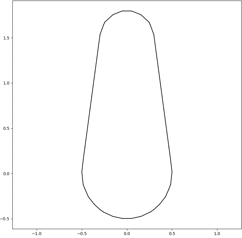
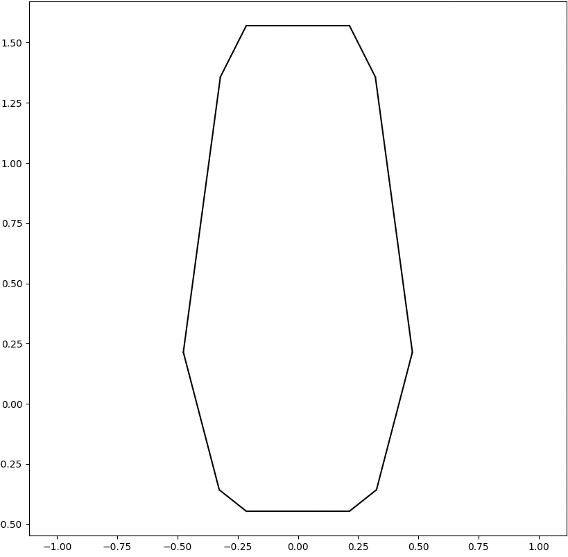
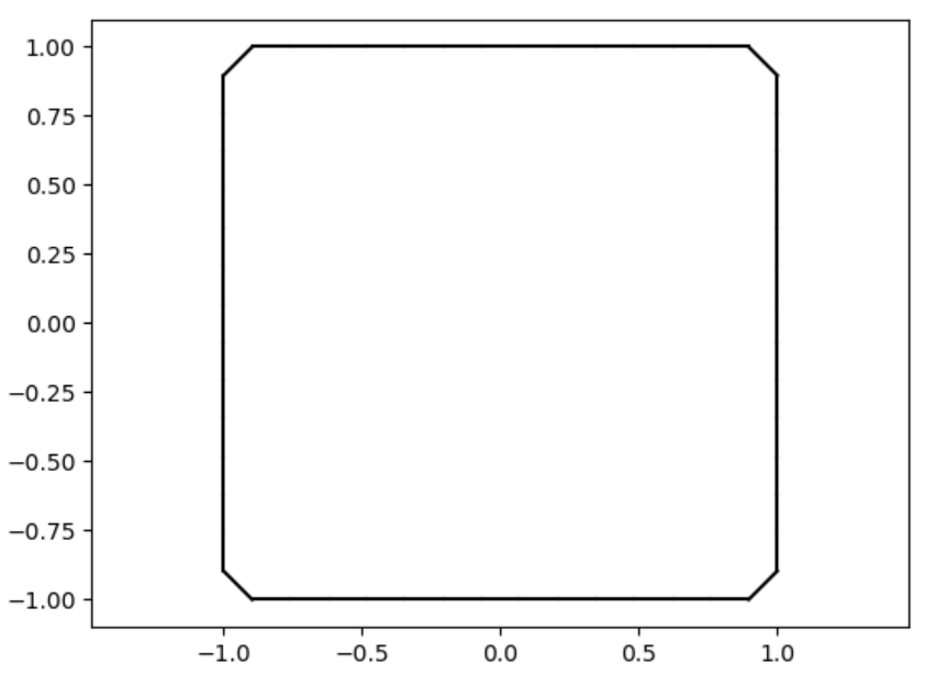
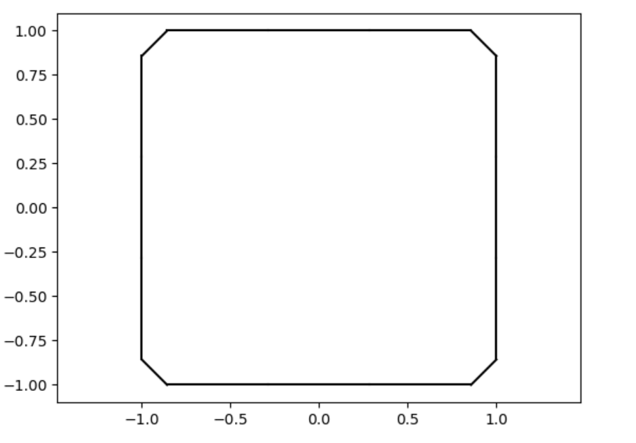
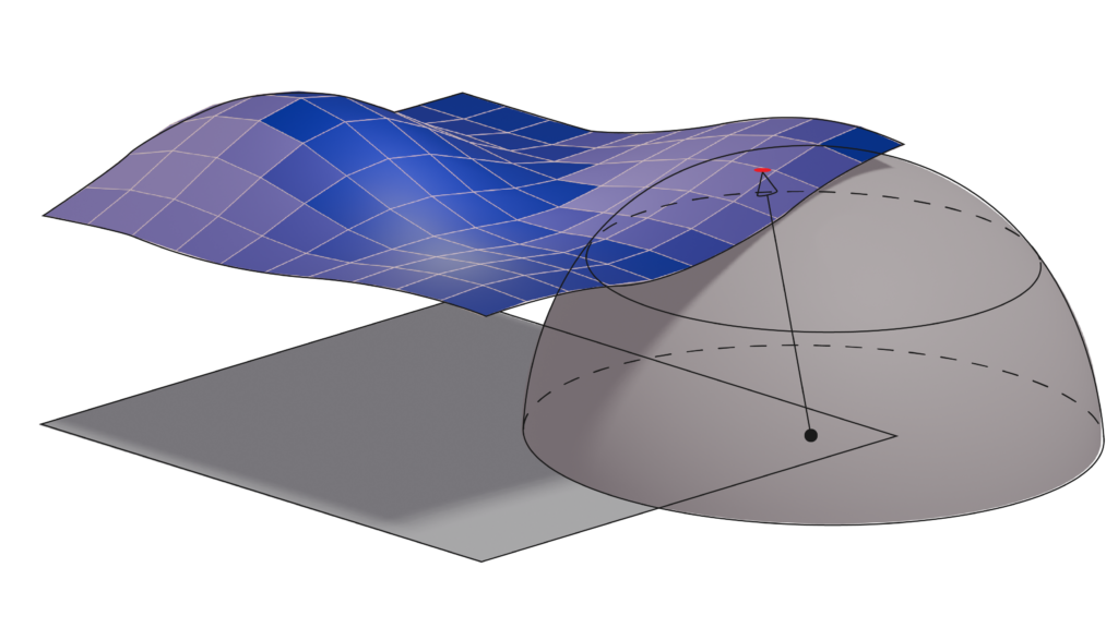
We analyze the Hausdorff distance for the uneven capsule (the shape on the right; exact sdf taken from there) in particular.

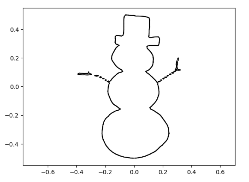
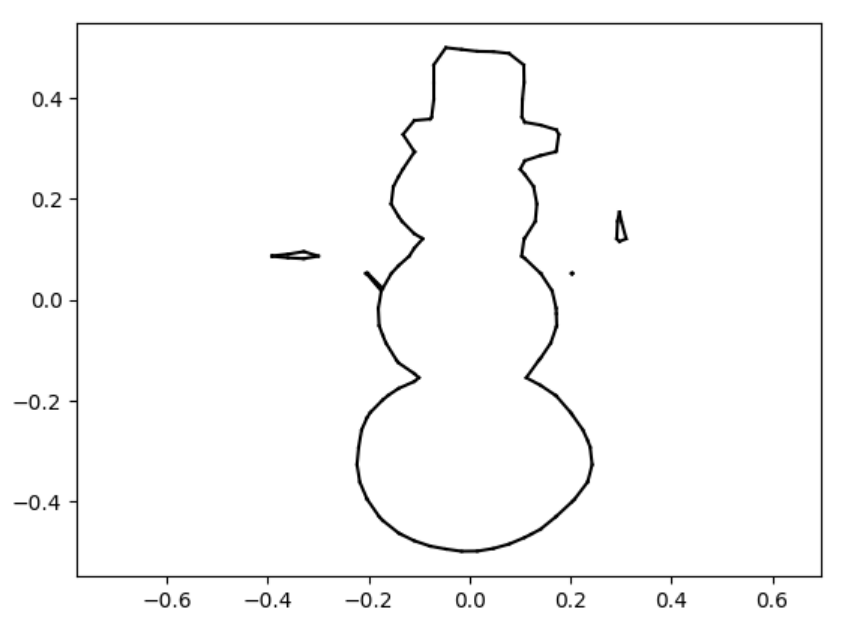
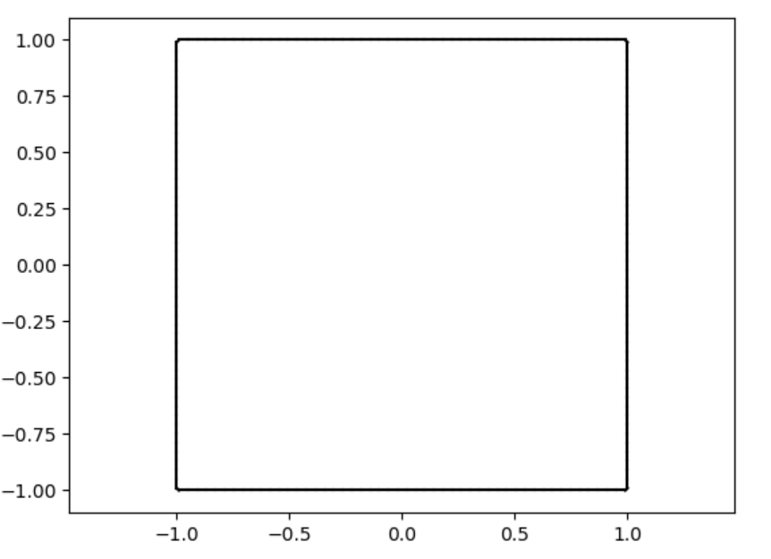
This plot visually compares the original zero level set (ground truth) with the reconstructed polyline generated by the marching squares algorithm at a specific resolution. The black dots represent the vertices of the polyline, showing how closely the reconstruction matches the ground truth, demonstrating the efficacy of the algorithm at capturing the shape’s essential features.

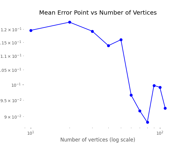
This plot shows the relationship between the Hausdorff distance and the resolution of the reconstruction. As resolution increases, the Hausdorff distance decreases, illustrating that higher resolutions produce more accurate reconstructions. The log-log plot with a linear fit suggests a strong inverse relationship, with the slope indicating a nearly quadratic decrease in Hausdorff distance as resolution improves.

Area Method for Error

Another error method we explored in this project is an area-based method. To start this process, we can overlay the original polyline and the generated polyline. Then, we can determine the area between the two, counting all regions as positive area. Essentially, this means that if we take values inside a polyline to be negative and outside a polyline to be positive, the area counted as error consists of the set of all regions where the sign of the original polyline’s SDF is not equal to the sign of the generated polyline’s SDF. The resultant area corresponds to the error of the reconstruction.

Here is a simple example of this area method using two quadrilaterals. The area between them is represented by their union (all blue area) with their intersection (the darker blue triangle) removed:

Here is an example of the area method applied to a star, with the area quantity corresponding to error printed at the top:

Inherent Error Function

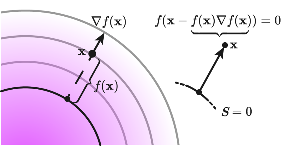
We define the error function between the reconstructed polyline and the zero level set (ZLS) of a given signed distance function (SDF) as:
$$
\mathrm{Error}=\frac{1}{|S|} \sum_{s \in S} \mathrm{sdf}(s)
$$

Here, \(S\) represents a set of sample points from the reconstructed polyline generated by the marching squares algorithm, and \(|\mathrm{S}|\) denotes the cardinality of this set. The sample points include not only the vertices but also the edges of the reconstructed polyline.

The key advantage of this error function lies in its simplicity and directness. Since the SDF inherently encodes the distance between any query point and the original polyline, there’s no need to compute distances separately as required in Hausdorff or Chamfer distance calculations. This makes the error function both efficient and well-suited to our specific context, providing a more streamlined and integrated approach to measuring the accuracy of the reconstruction.

Note that one variant one can consider is to square the \(\mathrm{sdf}(s)\) part to get rid of the signed nature, because the signs can cancel with each other for the reconstructed polyline is not always entirely inside the ground truth or entirely cotains the ground truth.

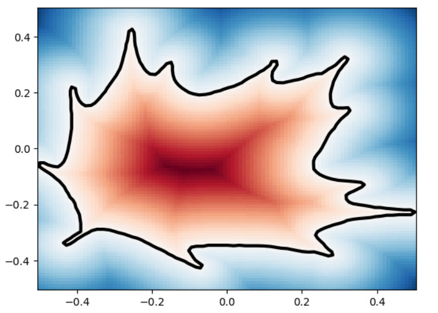
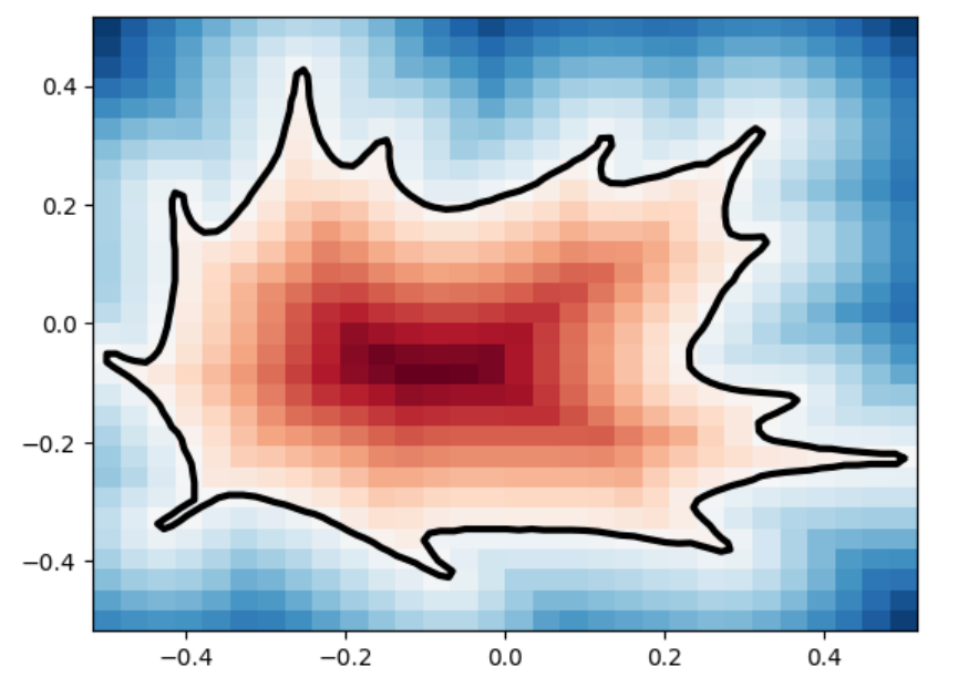
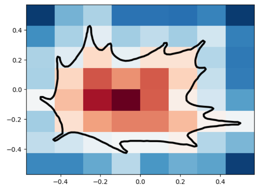
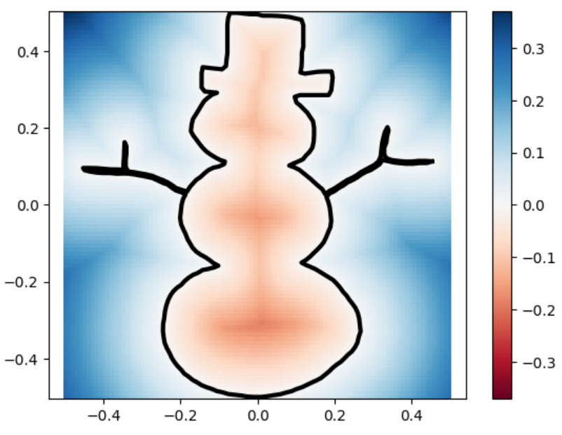
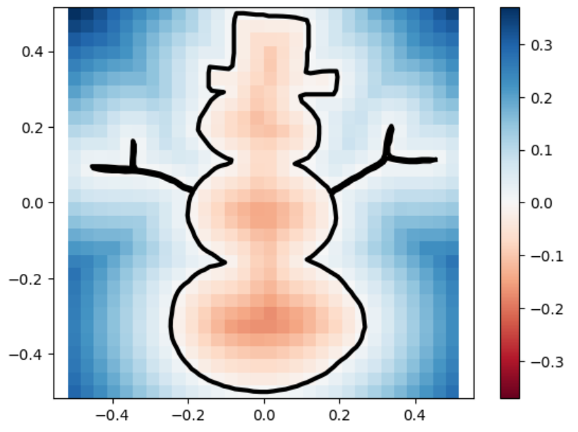
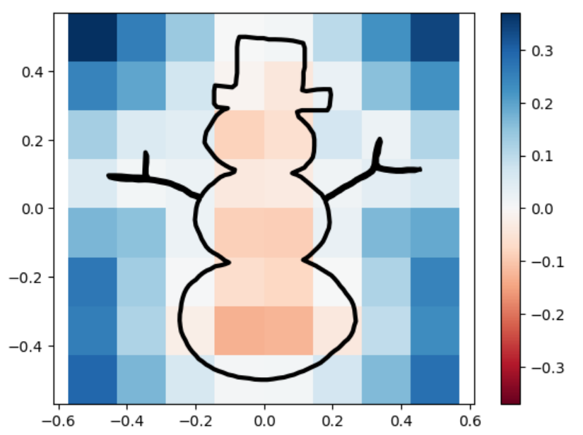
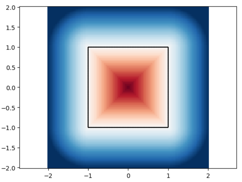
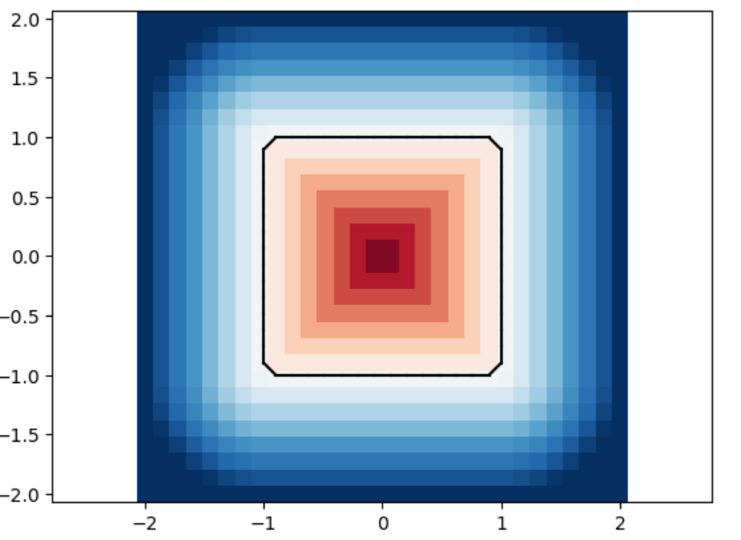
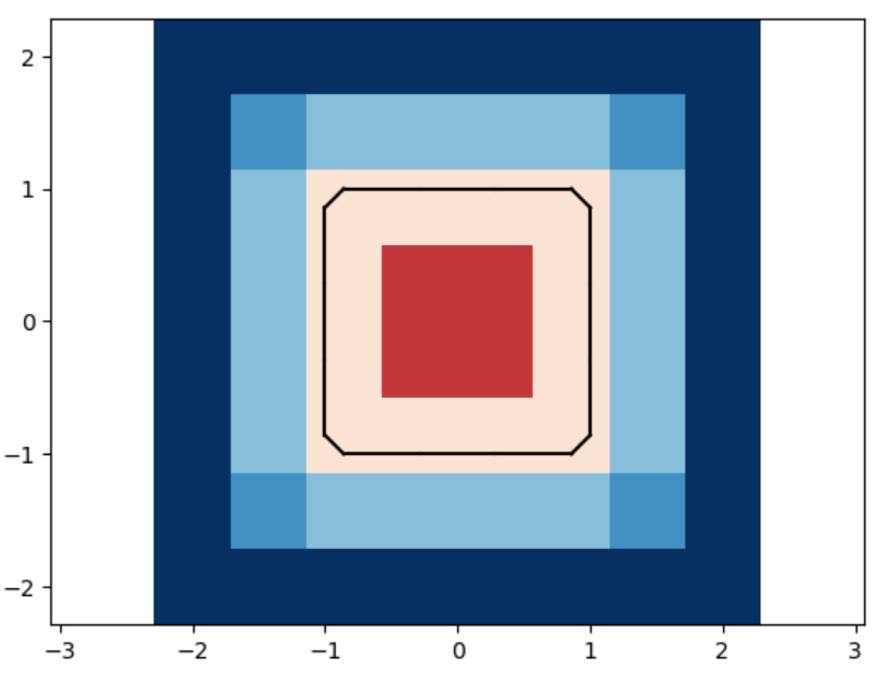
Below are one experiment we did for computing using this inherent error function, the unsquared one. We let the circle sdf be fixed and let the square sdf “escape” from the circle in a constant speed of \(0.2\). That is, we used the union of a fixed circle and a square with changing position as a series of shapes to do analysis. We then draw with color map used in this repo for the ground truths and the marching square results using the common color map.

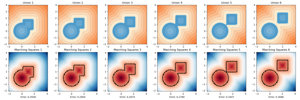
The inherent error of each union After several trials, one simple observation drawn from this escapaing motion is that when two shapes are more confounding with each other, as in the initial stage, the error is higher; and when the image starts to have two separated connected components, the error rises again. The first one can perhaps be explained by what the paper pointed out as pseudo-sdfs, and the second one is perhaps due to occurence of multipal components.

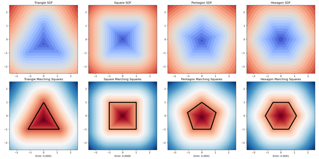
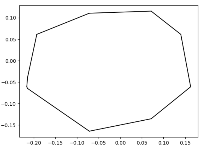
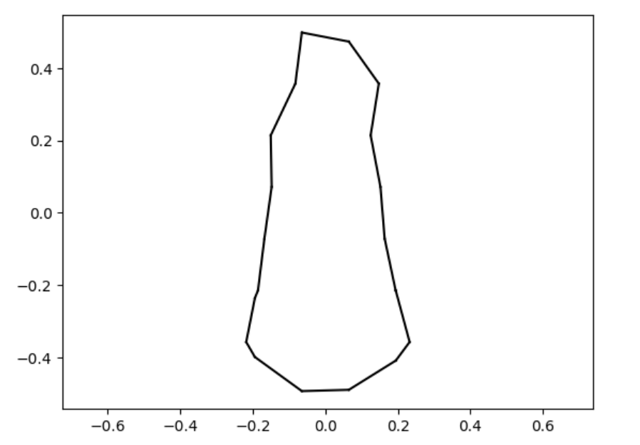
Here is another experiment. We want to know how well this method can simulate the physical characteristics of an object’s rugged level. We used a series of regular polygons. Although the result is theoretically unintheresting as the errors are all nearly zero, this is visually conformting.

Categories
Uncategorized

What’s a Neural Function?

Butlerian concerns aside, neural networks have proven to be extremely useful in doing everything we couldn’t think was to be done in this century; extremely advanced language processing, physically motivated predictions, and making strange, artful images using the power of bankrupt corporate morality.

Now, I’ve read and seen a lot of this “stuff” in the past, but I never really studied it, in-depth. Luckily, I got put with four exceedingly capable people in the area, and now manage to write a tabloid on the subject. I’ll write down the very basics of what I learned this week.

Taylor’s theorem

Suppose we had a function \( f : F \rightarrow L \) between the feature space \(F\) and a label space \(L\), both of these spaces are composed of a finite set of data points \( x_i \) and \( y_i \), we’ll put them into a dataset \(\mathfrak{D} = \{(x_i, y_i,) \}^N_{i=1} \). This function can represent just about anything as long as we’re capable of identifying the appropriate labels; images, videos and weather patterns.

The issue is, we don’t know anything about \(f\), but we do have a lot of data, so can we construct a arbitrarily good approximation \( f_\theta \) that functions a majority of the time? The whole field of machine learning asks not only if this is possibly, but if it is, how does one produce such a function, and with how much data?

Indeed, such a mapping may be extremely crooked, or of a high-dimensional character, but as long as we’re able to build universal function approximators of arbitrary precision, we should, in principle, be able to construct any such function.

Third-order Taylor approximation for the cubic polynomial \( x^3/7 + cos(x) \) around the point \( x = 3 \).

Naively, the first type of function approximator is a machine that produces a Taylor expansion; we call this machine \( f_\delta(\mathbf{x;w}) \) that approximates the real \( f(\mathbf{x})\). It contains the function input \( \mathbf{x}\), and a weight vector \(\mathbf{w}\) containing all of the coefficients of the Taylor expansion. We’ll call this parameter list the weights of the expansion.

Indeed, this same process can be taken up by any asymptotic series that converges onto the result. Now, what we’ve done is that we already had the function and wanted to find this approximation. Can we do the reverse procedure of acquiring a generic third degree polynomial: \[ f_\delta(x) = c_0 + c_1x + c_2 x^2 + c_3 x^3 \]

And then find the weights such that around the chosen point \( \mathbf{x} \) it fits with minimal loss? This question if of course, a extensively studied area of mathematically approximating/interpolating/extrapolating functions, and also the motivating factor for a NN, they’re effectively more complicated versions of this idea using a different method of fitting these weights, but it’s the same principle of applying a arbitrarily large number of computations to get to some range of values.

The first issue is that the label and feature spaces are enormously complicated, their dimensionality alone poses a formidable challenge in making a process to adjust said weights. Further, the structure in many of these spaces is not captured by the usual procedures of approximation. Taylor’s theorem, as our hanged man, is not capable of approximating very crooked functions, so that alone discards it, but

Thought(Thought(Thought(…)))

A neural network is the graphic representation of our neural function \(f_\theta\). We will define two main elements: a simple affine transform \(L = \mathbf{A}_i \mathbf{x} + \mathbf{b}_i \), and a activation function \( \sigma(L\), which can be any function, really, including a polynomial, but we often use a particular set of functions that are useful for NNs, such as a ReLu or a sigmoidal activation.

We can then produce a directed graph that shows the flow of computations we perform on our input \( \mathbf{x}\) across the many neurons of this graph. In this basic case, we have that the input \(x\) is feed onto two distinct neurons. The first transformation is \( \sigma_1(A_1x+b_1) \), whose result, \(x_1\), is feed onto the next neuron; the total result is a composition of the two transforms \(f \circ g = \sigma_2(A_2(f)+b_2 = \sigma_2(A_2(\sigma_1(A_1x+b_1))+b_2) \).

The total result of this basic net on the right is then \(\sigma_3(z) + \sigma_5(w) \), where \(w\) is the result of the transformations in the left, and \(z\) the ones on the right. We could do a labeling procedure and see then that the end result is of the form of a direct composition across the right layer of the affine transforms \((A, B, C)\) and activation functions \( (\sigma_1, \sigma_2, \sigma_3 \), and of the left hand side affine transforms \( (D, E, F) \) and functions \( (\sigma_4, \sigma_5, \sigma_6 ) \), which provides a 12-dimensional weight vector \( \mathbf{w} \):

\[ f_\theta(\mathbf{x;w}) = (\sigma_3\circ C \circ \sigma_2 \circ B \circ \sigma_1 \circ A) + (\sigma_6 \circ F \circ \sigma_5 \circ E \circ \sigma_4 \circ D) \]

Once again, the idea is that we can retrofit the coefficients of the affine transforms and activation functions to express different function approximations; different weight vectors yield different approximations. Finding the weights is called the training of the network and is done by an automatic process.

A feed forward NN is a deep, meaning it has more than intermediate layer, neural function \( f_\theta(\mathbf{x;w}) \) that, given some affine transformation \(f\) and activation function \(f\), is defined by:

\[ f_\theta(\mathbf{x;w}) = f_{n+1} \circ \sigma _n \circ f_n \circ \cdots \sigma_1\circ f_1 : \mathbb{R}^{n} \rightarrow \mathbb{R}^{n+1} \]

Here we see a basic FF neural function \( f_\theta (\mathbf{x, w}) \) and its corresponding neural network representation; it has a depth of 4 and a width of 3. The input \( x\) is feed into a singular neuron, that doesn’t change it, and its then feed to three distinct neurons, each with its own weights for the affine transformation, and this all repeats until the last neuron. All of them have the same underlying activation function \( \phi\):

If we actually go out and compute this particular neural function using \( \phi \) as the sigmoid function, we get the approximation of a sine wave. Therefore, we have sucessfully approximated a low dimensional function using a NN How did we, however, get these specifics weights? By means of gradient descent. Maybe I’ll write something about the trainings of NNs as I learn more about them.

Equivariant NNs

Now that we approximated a simple sine wave, the obvious next step is the three dimensional reconstruction of a mesh into a signed distance function.

But since I don’t actually know the latter, I’ll go to the non-obvious next step of looking at the image of an apple. If we were to perform a transformation on said apple as either a translation, rotation, or scaling, ideally our neural network should be able to still identify the data as an apple. This means we somehow need to encode the symmetry information onto the weights of the network. This breeds the principle of an equivariant NN, studied in the field of geometrical deep learning.

I’ll try to study these later to make more sense about them as well.

Categories
Research

A Study on Surface Reconstruction from Signed Distance Data Part 1: SDFs

Primary mentors:  Silvia Sellán, University of Toronto and Oded Stein, University of Southern California

Volunteer assistant:  Andrew Rodriguez

Fellows: Johan Azambou, Megan Grosse, Eleanor Wiesler, Anthony Hong, Artur, Sara  

The definition of SDFs using ducks

Suppose that you took a piece of metal wire, twisted into some shape you like, let’s make it a flat duck, and then put it on a little pond. The splash of water made by said wire would propagate as a wave all across the pond, inside and outside the wire. If the speed of the wave were \(1 m/s \), you’d have, at every instant, a wavefront telling you exactly how far away a given point is from the wire.

This is the principle behind a distance field, a scalar valued field \( d(\mathbf{x}) \) whose value at any given point \(\mathbf{x}\) is given by \( d(\mathbf{x}, S) = \min_{\mathbf{y}}d(\mathbf{x}, \mathbf{y})\), where \( S \) is a simpled closed curve. To make this a signed distance field, we can distinguish between the interior and exterior of the shape by adding a minus sign in the interior region.

Suppose we were to define sdf without knowing the boundary \(S\); given a region \( \Omega \) and a surface \( S \), whose inside is defined as the closure of \( \overline{\Omega} = A \). A function \( f : \mathbb{R}^n \rightarrow \mathbb{R} \) is said to be a signed distance function if for every point \( \mathbf{x} \in \Omega \) , we have eikonality \( | \nabla f | = 1 \) and closest point condition:
\[ f( \mathbf{x} – f(\mathbf{x}) \nabla f(\mathbf{x})) = 0 \]

The statement reads very simply: if we have a point \( \mathbf{x} \), and take the difference vector to the normal of the level set at hand times the distance, it should take us to the point \( \mathbf{x} \) closest to the zero level set.

This second definition is equivalent to the first one by an observation that eikonality implies \(1\)-Lipschitz property of the function \(f\) and it is also used for the last step of the following derivation: \(\exists q \in S:=f^{-1}(0)\)
$$
p-f(p) \nabla f(p)=q \Longrightarrow p-q=f(p) \nabla f(p) \Longrightarrow|p-q|=|f(p)|
$$

This combined with \(1\)-Lipschitz property gives a proof of contradiction for characterization of sdf by eikonality and closest point condition.

Our project was focused on the SDF-to-Surface reconstruction methods, which is, given a SDF, how can we make a surface out of it? I’ll first tell you about the much simpler problem, which is Surface-to-SDF.

Our SDFs

To lay the foundation, we started with the 2D case: SDFs in the plane from which we can extract polylines. Before performing any tests, we needed a database of SDFs to work with. We created our SDFs using two different skillsets: art and math.

The first of our SDFs were hand-drawn, using an algorithm that determined the closest perpendicular distance to a drawn image at the number of points in a grid specified by the resolution. This grid of distance values was then converted into a visual representation of these distance values – a two-dimensional SDF. Here are some of our hand-drawn SDFs!

The second of our SDFs were drawn using math! Known as exact SDFs, we determined these distances by splitting the plane into regions with inequalities and many AND/OR statements. Each of these regions was then assigned an individual distance function corresponding to the geometry of that space. Here are some of our exact SDF functions and their extracted polylines!

Exact vs. Drawn

Exact Signed Distance Functions (SDFs) provide precise, mathematically rigorous measurements of the shortest distance from any point to the nearest surface of a shape, derived analytically for simple forms and through more complex calculations for intricate geometries. These are ideal for applications demanding high precision but can be computationally intensive. Conversely, drawn or approximate SDFs are numerically estimated and stored in discretized formats such as grids or textures, offering faster computation at the cost of exact accuracy. These are typically used in digital graphics and real-time applications where speed is crucial and minor inaccuracies in distance measurements are acceptable. The choice between them depends on the specific requirements of precision versus performance in the application.

Operations on SDFs

For two SDFs, \(f_1(x)\) and \(f_2(x)\), representing two shapes, we can define the following operations from constructive geometry:

Union
$$
f_{\cup}(x) = \min(f_1(x), f_2(x))
$$

Intersection
$$
f_{\cap}(x) = \max(f_1(x), f_2(x))
$$

Difference
$$
f_{\setminus}(x) = \max(f_1(x), -f_2(x))
$$

We used these operations to create the following new sdfs: a cat and a tessellation by hexagons.

Marching Squares Reconstructions with Multiple Resolutions

The marching_squares algorithm is a contouring method used to extract contour lines (isocontours) or curves from a two-dimensional scalar field (grid). It’s the 2D analogue of the 3D Marching Cubes algorithm, widely used for surface reconstruction in volumetric data. When applied to Signed Distance Functions (SDFs), marching_squares provides a way to visualize the zero level set (the exact boundary) of the function, which represents the shape defined by the SDF. Below are visualizations of various SDFs which we passed into marching squares with varied resolutions in order to test how well it reconstructs the original shape.

SDF / Resolution100×10030×308×8
leaf
leaf
marching_squares
uneven capsule
uneven capsule marching_squares
snowman
snowman marching_squares
square
square
marching_squares
sdfs and reconstructions in three different resolutions.

SDFs in 3D Geometry Processing

While the work we have done has been 2D in our project, signed-distance functions can be applied to 3D geometry meshes in the same way. Below are various examples from recent papers that use signed distance functions in the 3D setting. Take for example marching cubes, a method for surface reconstruction in volumetric data developed by Lorensen and Cline in 1987 that was originally motivated by medical imaging. If we start with an implicit function, then the marching cubes algorithm works by “marching” over a uniform grid of cubes and then locating the surface of interest by seeing where the surface intersects with the cubes, and adding triangles with each iteration such that a triangle mesh can ultimately be formed via the union of each triangle. A helpful visualization of this algorithm can be found here

Take for example our mentors Silvia Sellán and Oded Stein’s recent paper “Reach For the Spheres:Tangency-Aware Surface Reconstruction of SDFs” with C. Batty which introduces a new method for reconstructing an explicit triangle mesh surface corresponding to an SDF, an algorithm that uses tangency information to improve reconstructions, and they compare their improved 3D surface reconstructions to marching cubes and an algorithm called Neural Dual Contouring. We can see from their figure below that their SDF and tangency-aware and reconstruction algorithm is more accurate than marching cubes or NDCx.

(From Sellan et al, 2024) The Reach for the Spheres method that using tagency information for more accurate surface reconstructions can be seen on both 10^3 and 50^3 SDF grids as being more accurate than competing methods of marching cubes and NDCx. They used features of SDF and the idea of tangency constraints for this novel algorithm.

Another SGI mentor, Professor Keenan Crane, also works with signed distance functions. Below you can see in his recent paper “A Heat Method for Generalized Signed Distance” with Nicole Feng, they introduce a novel method for SDF approximation that completes a shape if the geometric structure of interest has a corrupted region like a hole.

(From Feng and Crane, 2024): In this figure, you can see that the inputted curves in magenta are broken, and the new method introduced by Feng and Crane works by computing signed distances from the broken curves, allowing them to ultimately generate an approximated SDF for the corrupted geometry where other methods fail to do this.

Clearly, SDFs are beautiful and extremely useful functions for both 2D and 3D geometry tasks. We hope this introduction to SDFs inspires you to study or apply these functions in your future geometry-related research. 

References

Sellán, Silvia, Christopher Batty, and Oded Stein. “Reach For the Spheres: Tangency-aware surface reconstruction of SDFs.” SIGGRAPH Asia 2023 Conference Papers. 2023.

Feng, Nicole, and Keenan Crane. “A Heat Method for Generalized Signed Distance.” ACM Transactions on Graphics (TOG) 43.4 (2024): 1-19.

Marschner, Zoë, et al. “Constructive solid geometry on neural signed distance fields.” SIGGRAPH Asia 2023 Conference Papers. 2023.

Categories
Research

How to match the “wiggliness” of two shapes

If you have an object which you would like to represent as a mesh, what measure do you use to make sure they’re matched nicely?

Suppose you had the ideal, perfectly round implicit sphere \( || \mathbf{x}|| = c\), and you, as a clever geometry processor, wanted to make a discrete version of said sphere employing a polygonal mesh \( \mathbf{M(V,F)}\). The ideal scenario is that by finely tessellating this mesh into a limit of infinite polygons, you’d be able to approach the perfect sphere. However, due to pesky finite memory, you only have so many polygons you can actually add.

The question then becomes, how do you measure how well the perfect and tessellated spheres match? Further, how would you do it for any shape \( f(\mathbf{x}) \)? Is there also a procedure not just for perfect shapes, but also to compare two different meshes? That was the objective of Nicholas Sharp’s research program this week.

The 1D Case

Suppose we had a curve \( A(t):[0,1] \rightarrow \mathbb{R}^n \), and we want to build an approximate polyline curve
\( B(t) \). We want to make our discrete points have the nearest look to our original curve \( A(t) \).

As such, we must choose an error metric measuring how similar the two curves are, and make an algorithm that produces a curve that minimizes this metric. A basic one is simply to measure the total area separating the approximate and real curve, and attempt to minimize it.

The error metric for two curves is the area  between them

The distance between the polyline and the curve \( |A(t) – B(t)| \) is what allows us to produce this error functional, that tells us how much or how little they match. That’s all there is to it. But how do we compute such a distance?

Well, one way is the Chamfer Distance of the two sets of points \( ch(A,B) \). It’s defined as the nearest point distance among the two curves, and all you need to figure it out is to draw little circles along one of the curves. Where the circles touch defines their nearest point!

Here \( d(A,B) \) is just the regular Euclidean distance. Now we would only need to minimize a error functional proportional to \[ \partial E(A,B) = \int_{\gamma} ch(A,B) \sim \sum_{i=0}^n dL \ ch(A, B) = 0 \]

Well simple enough, but there’s a couple of problems. The first one is most evident: a “nearest point query” between curves does not actually contain much geometrical information. A simple counterexample is a spikey curve near a relatively flat curve; the nearest point to a large segment of the curve is a single peak!

We’ll see another soon enough, but this immediately brings into question the validity of an attempted approximation using \( ch(A,B) \). Thankfully mathematicians spent a long time idly making up stuff, so we actually have a wide assortment of possible distance metrics to use!

Different error metrics

The first alternative metric is the classic Hausdorff Distance, defined as upper bound of the Chamfer distance. Along a curve, always picking the smallest distances, we can select the largest such distance.

Where we to use such a value, the integral error would be akin to the mean error value, rather than the absolute total area. This does not fix our original shape problem, but it does facilitate computation!

The last contender for our curves is the Fréchet Distance. It is relatively simple: you parametrize two curves \( A \) and \( B \) by some parameter \( t \) such that \(A(\alpha(t)) \) and \( B(\beta(t))\), you can picture it as time; it is always increasing. What we do is say that Fréchet distance \( Fr(A,B) \) is the instantaneous distance between two points “sliding along” the two curves:

We can write this as \[ Fr(A, B) = \inf_{\alpha, \beta} \max_{t\in[0,1]} d(A(\alpha(t)), B(\beta(t))) \]

This provides many benefits at the cost of computation time. The first is that it immediately corrects points from one of our curves “sliding back” as in the peak case, since it must be a completely injective function in the sense one point at some parameter \( t \) must be unique.

The second is that it encodes shape data. The shape information is contained in the relative distribution of the parametrization; for example, if we were to choose \( \alpha(t) \approx \ln t \), we’d produce more “control points” at the tail end of the curve and that’d encode information about its derivatives. The implication being that this information, if associated to the continuity \( (C^n) \) of the curve, could imply details of its curvature and such.

Here is a simple example. Suppose we had two very squiggly curves criss-crossing each other:

Now, were we to choose a Chamfer/Hausdorff distance variant, we would actually get a result indicating a fairly low error, because, due to the criss-cross, we always have a small distance to the nearest point:

However, were we to introduce a parametrization along the two curves that is roughly linear, that is, equidistant along arclenghts of the curve, we could verify that their Fréchet distance is very large, since “same moment in time” points are widely distanced:

Great!

The 2D case

In our experiments with Nicholas, we only got as far as generalizing this method to disk topology, open grid meshes, and using the Chamfer approach to them. We first have a flat grid mesh, and apply a warp function \( \phi(\mathbf{x}) \) that distorts it to some “target” mesh.

def warp_function(uv):

    # input: array of shape (n, 2) uv coordinates. (n,3) input will just ignore the z coordinate

    ret = []
    for i in uv:
        ret.append([i[0], i[1], i[0]*i[1]])

    return np.array(ret)

We used a couple of test mappings, such as a saddle and a plane with a logarithmic singularity.

We then do a Chamfer query to evaluate the absolute error by summing all the distances from the parametric surface to the grid mesh. The 3D Chamfer metric is simply the nearest sphere query to a point in the mesh:

def chamfer_distance(A, B):
    ret = 0
    closest_points = []

    for a in range(A.shape[0]):
        min_distance = float('inf')
        closest_point = None
        for b in range(B.shape[0]):
            distance = np.linalg.norm(A[a] - B[b])
            if distance < min_distance:
                min_distance = distance
                closest_point = b
        ret += min_distance
        closest_points.append((a, A.shape[0]+closest_point))
    
    closest_points_vertices = np.vstack([A, B])
    closest_points_indices = np.array(closest_points)

    assert closest_points_indices.shape[0] == A.shape[0] 
and closest_points_indices.shape[1] == 2
    assert closest_points_vertices.shape[0] == A.shape[0] + B.shape[0] and closest_points_vertices.shape[1] == A.shape[1]

    return ret, closest_points_vertices, closest_points_indices

Our main goals were to check if, as the base grid mesh was refined, the error diminished as the approximation increased in resolution, and to see if the relative angle of the grid mesh to the test function significantly altered the error.

The first experiment was validated quite successfully; besides perhaps very pathological cases, the error diminished as we increased the resolution:

And the second one as well, but this will be discussed in a separate blog post.

Application Areas: Chamfer Loss in Action

In machine learning, a loss function is used to measure the difference (i.e. error) between the given input and the neural network’s output. By following this measure, it is possible to have an estimate of how well the neural network models the training data and optimize its weights with respect to this.

For the task of mesh reconstruction, e.g. reconstructing a surface mesh given an input representation such as a point cloud, the loss function aims to measure the difference between the ground truth and predicted mesh. To achieve this, the Chamfer loss (based on the Chamfer distance discussed above) is utilized.

Below, we provide a code snippet for the implementation of Chamfer distance from a widely adopted deep learning library for 3D data, PyTorch3D [1]. The distance can be modified to be used as single or bi-directional (single_directional) and by adopting additional weights.

def chamfer_distance(
    x,
    y,
    x_lengths=None,
    y_lengths=None,
    x_normals=None,
    y_normals=None,
    weights=None,
    batch_reduction: Union[str, None] = "mean",
    point_reduction: Union[str, None] = "mean",
    norm: int = 2,
    single_directional: bool = False,
    abs_cosine: bool = True,

):

    if not ((norm == 1) or (norm == 2)):

        raise ValueError("Support for 1 or 2 norm.")

    x, x_lengths, x_normals = _handle_pointcloud_input(x, x_lengths, x_normals)

    y, y_lengths, y_normals = _handle_pointcloud_input(y, y_lengths, y_normals)

    cham_x, cham_norm_x = _chamfer_distance_single_direction(
        x,
        y,
        x_lengths,
        y_lengths,
        x_normals,
        y_normals,
        weights,
        batch_reduction,
        point_reduction,
        norm,
        abs_cosine,
    )
    if single_directional:
        return cham_x, cham_norm_x

    else:
        cham_y, cham_norm_y = _chamfer_distance_single_direction(

            y,
            x,
            y_lengths,
            x_lengths,
            y_normals,
            x_normals,
            weights,
            batch_reduction,
            point_reduction,
            norm,
            abs_cosine,
        )

        if point_reduction is not None:
            return (
                cham_x + cham_y,
                (cham_norm_x + cham_norm_y) if cham_norm_x is not None else None,
            )
        return (
            (cham_x, cham_y),
            (cham_norm_x, cham_norm_y) if cham_norm_x is not None else None,

        )

When Chamfer is not enough

Depending on the task, the Chamfer loss might not be the best measure to estimate the difference between the surface and reconstructed mesh. This is because in certain cases, the \( k \)-Nearest Neighbor (KNN) step will always be taking the difference between the input point \( \mathbf{y} \) and the closest point \( \hat{\mathbf{y}}\) on the reconstructed mesh, leaving aside the actual point where the measure should be taken into account. This could lead a gap between the input point and the reconstructed mesh to stay untouched during the optimization process. Research for machine learning in geometry proposes to adopt different loss functions to mitigate this problem introduce by the Chamfer loss.

A recent work Point2Mesh [2] addresses this issue by proposing the Beam-Gap Loss. For a point \( \hat{\mathbf{y}}\) sampled from a deformable mesh face, a beam is cast in the direction of the deformable face normal. The beam intersection with the point cloud is the closest point in an \(\epsilon\) cylinder around the beam. Using a cylinder around the beam instead of a single point as in the case of Chamfer distance helps reduce the gap in a certain region between the reconstructed and input mesh.

The beam intersection (or collision) of a point \( \hat{\mathbf{y}}\) is formally given by \( \mathcal{B}(\hat{\mathbf{y}}) = \mathbf{x}\) and the overall beam-gap loss is calculated by:

\[ \mathcal{L}_b (X, \hat{\mathbf{Y}}) = \sum_{ \hat{y} \in \hat{Y}} |\hat{\mathbf{y}}-\mathcal{B}(\hat{\mathbf{y}})|^2 \]

References

[1] Ravi, Nikhila, et al. “Accelerating 3d deep learning with pytorch3d.” arXiv preprint arXiv:2007.08501 (2020).

[2] Hanocka, Rana, et al. “Point2mesh: A self-prior for deformable meshes.” SIGGRAPH (2020).

[3] Alt, H., Knauer, C. & Wenk, C. Comparison of Distance Measures for Planar Curves. Algorithmica

[4] Peter Schäfer. Fréchet View – A Tool for Exploring Fréchet Distance Algorithms (Multimedia Exposition).

[5] Aronov, B., Har-Peled, S., Knauer, C., Wang, Y., Wenk, C. (2006). Fréchet Distance for Curves, Revisited. In: Azar, Y., Erlebach, T. (eds) Algorithms

[6] Ainesh Bakshi, Piotr Indyk, Rajesh Jayaram, Sandeep Silwal, and Erik Waingarten. 2024. A near-linear time algorithm for the chamfer distance. Proceedings of the 37th International Conference on Neural Information Processing Systems.