Fellows: Mutiraj Laksanawisit, Diana Aldana Moreno, Anthony Hong
Our task is to fit closed and watertight surfaces to point clouds that might have a lot of noise and inconsistent outliers. There are many papers like this, where we will explore a modest variation on the problem: we will allow the system to modify the input point clouds in a controlled manner, where the modification will be gradually scaled back until the method fits to the original point clouds. The point of this experiment is to check whether such modification is beneficial for both accuracy and training time.
Regular Point-Cloud Fitting
A point clouds is an unordered set of 3D points: \(\mathscr{P}=\left\{x_i, y_i, z_i\right\}\), where \(0<i\leq N\) for some size \(N\). These points can be assumed to be accompanied by normals \(n_i\) (as unit vectors associated to each points). An \emph{implicit} surface reconstruction tries to fit a function \(f(x,y,z)\) to every point in space, such that its zero set $$ S = f^{-1}(0)=\left\{(x,y,z) | f(x,y,z)=0\right\} $$ represents the surface.
We usually train \(f\) to be a signed distance function (SDF) \(\mathbb{R}^3\rightarrow\mathbb{R}\) from the zero set. That is, to minimize the loss: $$ f = \text{argmin}\left(\lambda_{p}E_p+\lambda_{n}E_n+\lambda_{s}E_s\right) $$
where \begin{align} E_p &= \sum_{i=0}^N{|f(x_i,y_i,z_i)|^2}\\ E_n &= \sum_{i=0}^N{|\nabla f(x_i,y_i,z_i)-n_i|^2}\\ E_s &= \sum_{j=0}^Q{||\nabla f(x_j,y_j,z_j)|-1|^2} \end{align} Loss term \(E_p\) is for the zero-set fitting. Loss term \(E_n\) is for the normal fitting, and term \(E_s\) is for regulating \(f\) to be an SDF; it is trained on a randomly sampled set \(\mathscr{Q}=\left(x_j,y_j,z_j\right)\) (of size \(Q=|\mathscr{Q}|\)) in the bounding box of the object, that gets replaced every few iterations. The bounding box should be a bit bigger, say cover %20 more in each axis, to allow for enough empty space around the object.
Reconstruction Results
We extracted meshes from this repository and apply Poisson disc sampling with point-number parameter set at 1000 (but note that the resulted sampled points are not 1000; see the table below) on MeshLab2023.12. We then standardize the grids and normalize the normals (the xyz file with normals does not give normals in this version of MeshLab so we need to an extra step of normalization). Then we ran the learning procedure on these point clouds to fit an sdf with 500 epochs and other parameters shown below.
We then plots the results (the neural netwok, the poitclouds and normals) and registered isosurfaces as meshes on polyscope and used slice planes to see how good are the fits. Check the table below.
Nefertiti
Homer
Kitten
Original meshes
Vertices of sample
1422
1441
1449
Reconstructions
slice 1
slice 2
slice 3
slice 4
slice 5
slice 6
Reconstruction results of Nefertiti.obj, Homer.obj, and Kitten.obj.
Ablation Test
There are several parameters and methods we can play around. Basically, we did not aim to prove for some “optimal” set of parameters. Our approach is very experimental: we tried different set of parameters (learning rate, batch size, epoch number, and weights of each energy term) and see how good is the fit for each time we changed the set. If the results look good then the set is good, and the set we chose is included in the last subsection. We used the ReLU activation function and the results are generally good. We also tried tanh, which gives smoother reconstructed surfaces.
Adversarial Point Cloud Fitting
First try to randomly add noise to the point cloud of several levels, and try to fit again. You will see that the system probably performs quite poorly. Do so by adding a \(\epsilon_i\) to each point \((x_i,y_i,z_i)\) of a small Gaussian distribution. Test the result, and visualize it to several variances of noise.
We’ll next reach the point of the project, which is to learn an adversarial noise. We will add another module \(\phi\) that connects between the input and the network, where: $$ \phi(x,y,z) = (\delta, p) $$ \(\phi\) outputs a neural field \(\delta:\mathbb{R}^3\rightarrow \mathbb{R}^3\), that serves as a perturbation of the point clouds, and another neural field \(p:\mathbb{R}^3\rightarrow [0,1]\) that serves as the confidence measure of each point. Both are fields; that is they are defined ambiently in \(\mathbb{R}^3\), but we’ll use their sampling on the points \(\mathscr{P}_i\). Note that \(f\) is the same way!
The actual input to \(f\) is then \((x,y, z)+\delta\), where we extend the network to also receive \(p\). We then use the following augmented loss: $$ f = \text{argmin}\left(\lambda_{p}\overline{E}_p+\lambda_{n}\overline{E}_n+\lambda_{s}\overline{E}_s +\lambda_d E_d + \lambda_v E_v + \lambda_p E_p\right), $$ where \begin{align} E_d &= \sum_{i=0}^N{|\delta_i|^2}\\ E_v &= \sum_{i=0}^N{|\nabla \delta_i|^2}\\ E_p &= -\sum_{i=0}^N{log(p_i)}. \end{align} \(E_d\) regulates the magnitude of \(\delta\); it is zero if we try to adhere to the original point cloud. \(E_v\) regulates the smoothness of \(\delta\) in space, and \(E_p\) encourages the point cloud to trust the original points more, according to their confidences (it’s perfectly \(0\) when all \(p_i=1\). We use \(\delta_i=\delta(x_i,y_i,z_i)\) and similarly for \(p_i\).
The original losses are also modified according to \(\delta\) and \(p\): consider \(\overline{f} = f((x,y,z)+\delta)\), then: \begin{align} \overline{E}_p &= \sum_{i=0}^N{p_i|\overline{f}(x_i,y_i,z_i)|^2}\\ \overline{E}_n &= \sum_{i=0}^N{p_i|\nabla \overline{f}(x_i,y_i,z_i)-n_i|^2}\\ \overline{E}_s &= \sum_{j=0}^Q{||\nabla \overline{f}(x_j,y_j,z_j)|-1|^2} \end{align} By controlling the learnable \(\delta\) and \(p\), we aim to achieve a better loss; that essentially means smoothing the points and trusting those that are less noisy. This should result is quicker fitting, but less accuracy. We then, gradually with the iterations, try to increase \(\lambda_{d,v,p}\) more and more so to subdue \(\delta\) and trust the original point cloud more and more.
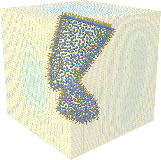
Reconstruction Results
We use a network with a higher capacity to represent the perturbations \(\delta\) and the confidence probability \(p\). Specifically, we define a \(2\)-hidden layer ReLU MLP with sine for the first activation layer. This allows to represent high frequency details necessary to approximate the noise \(\delta\).
During the experiments, we notice that the parameters \(\lambda_d\), \(\lambda_v\), and \(\lambda_p\) have different behaviors over the resulting loss. The term \(E_d\) converges easily, so the value for \(\lambda_d\) is chosen to be small. On the other hand, the loss \(E_v\) that regulates smoothness is harder to fit so we choose a bigger \(\lambda_v\). Finally, the term \(E_p\) is the most sensitive one since it is defined as a sum of logarithms, meaning that small coordinates of \(p\) may lead to \(\texttt{inf}\) problems. For this term, a not so big, not so small value must be chosen, so as to have a confidence parameter near \(1\) and still converge.
As we can see from the image below, our reconstruction still has a way to go, however, there are still many ideas we still could test: How do the architectures influence the training? Which is the best function to reduce the influence of the adversarial loss terms during training? Are all loss terms really necessary?
Overall this is an interesting project that allow us to explore possible solutions to noisy data in 3D, that it’s still far away from being completely explored.
Primary mentors: Silvia Sellán, University of Toronto and Oded Stein, University of Southern California
Volunteer assistant: Andrew Rodriguez
Fellows: Johan Azambou, Megan Grosse, Eleanor Wiesler, Anthony Hong, Artur RB Boyago, Sara Samy
After talking about what are some of the ways to reconstruct sdfs (see part one), we now study the question of how to evaluate their performance. Two classes of error function are considered, the first more inherent to our sdf context, and the second more general in all situations. We will first show results by our old friends, Chamfer distance, Hausdorff distance, and area method (see here for example), and then introduce the inherent one.
Hausdorff and Chamfer Distance
The Chamfer distance provides an average-case measure of the dissimilarity between two shapes. It calculates the sum of the distances from each point in one set to the nearest point in the other set. This measure is particularly useful when the goal is to capture the overall discrepancy between two shapes while being less sensitive to outliers. The Chamfer distance is defined as: $$ d_{\mathrm{Chamfer }}(X, Y):=\sum_{x \in X} d(x, Y)=\sum_{x \in X} \inf _{y \in Y} d(x, y) $$
The Bi-Chamfer distance is an extension that considers the average of the Chamfer distance computed in both directions (from \(X\) to \(Y\) and from \(Y\) to \(X\) ). This bidirectional measure provides a more balanced assessment of the dissimilarity between the shapes: $$ d_{\mathrm{B} \mathrm{-Chamfer }}(X, Y):=\frac{1}{2}\left(\sum_{x \in X} \inf {y \in Y} d(x, y)+\sum{y \in Y} \inf _{x \in X} d(x, y)\right) $$
The Hausdorff distance, on the other hand, measures the worst-case scenario between two shapes. It is defined as the maximum distance from a point in one set to the closest point in the other set. This distance is particularly stringent because it reflects the largest deviation between the shapes, making it highly sensitive to outliers.
The formula for Hausdorff distance is: $$ d_{\mathrm{H}}^Z(X, Y):=\max \left(\sup {x \in X} d_Z(x, Y), \sup {y \in Y} d_Z(y, X)\right) $$
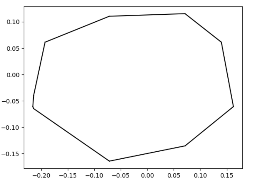
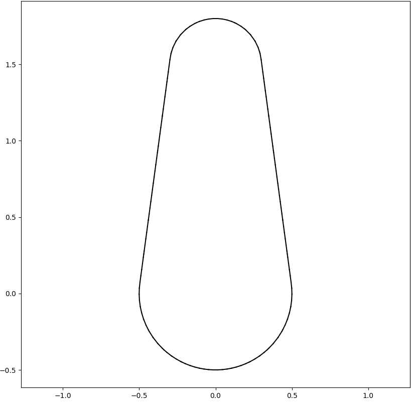
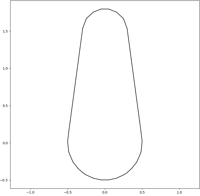
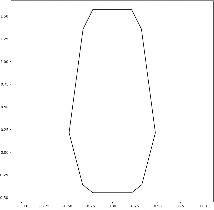
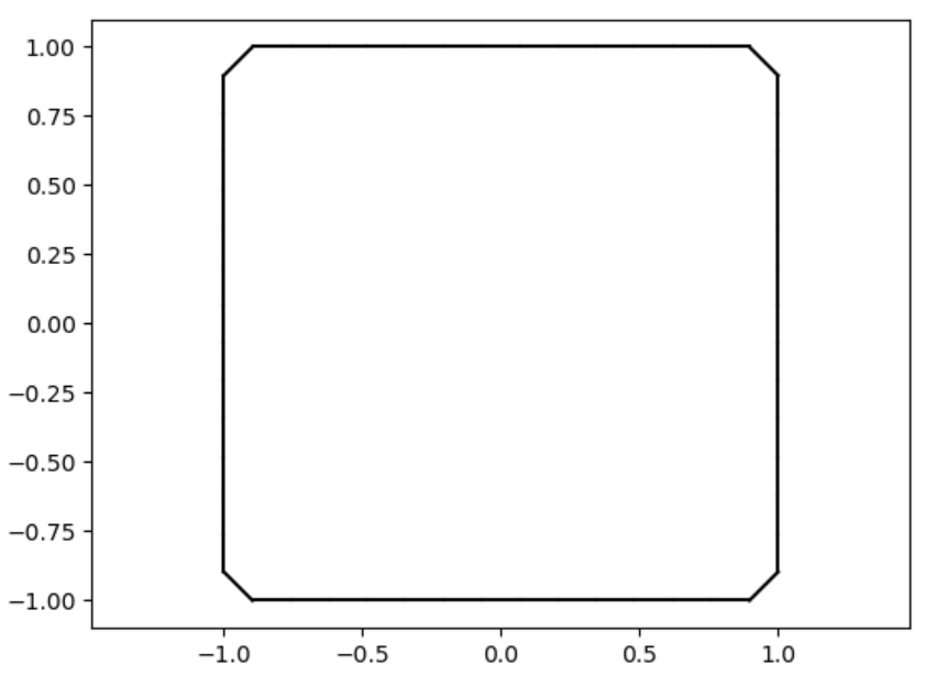
We analyze the Hausdorff distance for the uneven capsule (the shape on the right; exact sdf taken from there) in particular.
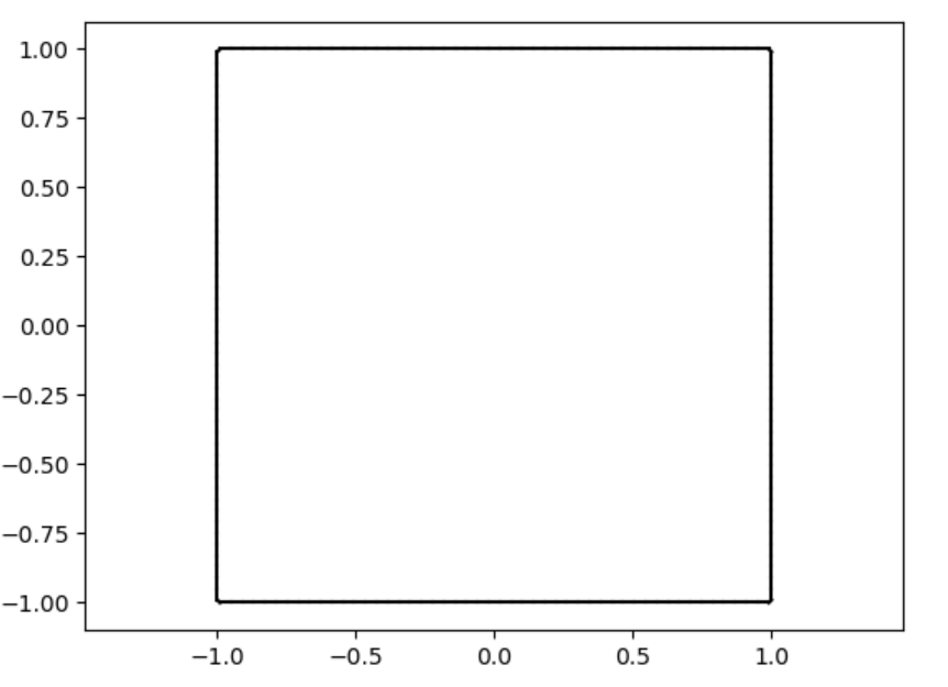
This plot visually compares the original zero level set (ground truth) with the reconstructed polyline generated by the marching squares algorithm at a specific resolution. The black dots represent the vertices of the polyline, showing how closely the reconstruction matches the ground truth, demonstrating the efficacy of the algorithm at capturing the shape’s essential features.
This plot shows the relationship between the Hausdorff distance and the resolution of the reconstruction. As resolution increases, the Hausdorff distance decreases, illustrating that higher resolutions produce more accurate reconstructions. The log-log plot with a linear fit suggests a strong inverse relationship, with the slope indicating a nearly quadratic decrease in Hausdorff distance as resolution improves.
Area Method for Error
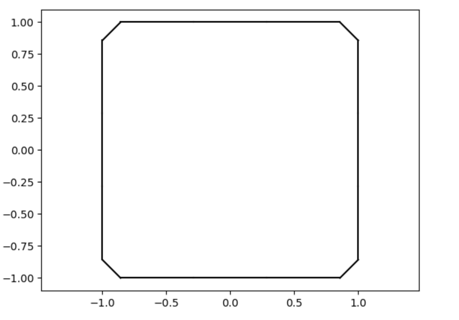
Another error method we explored in this project is an area-based method. To start this process, we can overlay the original polyline and the generated polyline. Then, we can determine the area between the two, counting all regions as positive area. Essentially, this means that if we take values inside a polyline to be negative and outside a polyline to be positive, the area counted as error consists of the set of all regions where the sign of the original polyline’s SDF is not equal to the sign of the generated polyline’s SDF. The resultant area corresponds to the error of the reconstruction.
Here is a simple example of this area method using two quadrilaterals. The area between them is represented by their union (all blue area) with their intersection (the darker blue triangle) removed:
Here is an example of the area method applied to a star, with the area quantity corresponding to error printed at the top:
Inherent Error Function
We define the error function between the reconstructed polyline and the zero level set (ZLS) of a given signed distance function (SDF) as: $$ \mathrm{Error}=\frac{1}{|S|} \sum_{s \in S} \mathrm{sdf}(s) $$
Here, \(S\) represents a set of sample points from the reconstructed polyline generated by the marching squares algorithm, and \(|\mathrm{S}|\) denotes the cardinality of this set. The sample points include not only the vertices but also the edges of the reconstructed polyline.
The key advantage of this error function lies in its simplicity and directness. Since the SDF inherently encodes the distance between any query point and the original polyline, there’s no need to compute distances separately as required in Hausdorff or Chamfer distance calculations. This makes the error function both efficient and well-suited to our specific context, providing a more streamlined and integrated approach to measuring the accuracy of the reconstruction.
Note that one variant one can consider is to square the \(\mathrm{sdf}(s)\) part to get rid of the signed nature, because the signs can cancel with each other for the reconstructed polyline is not always entirely inside the ground truth or entirely cotains the ground truth.
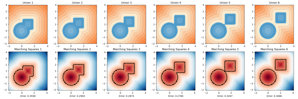
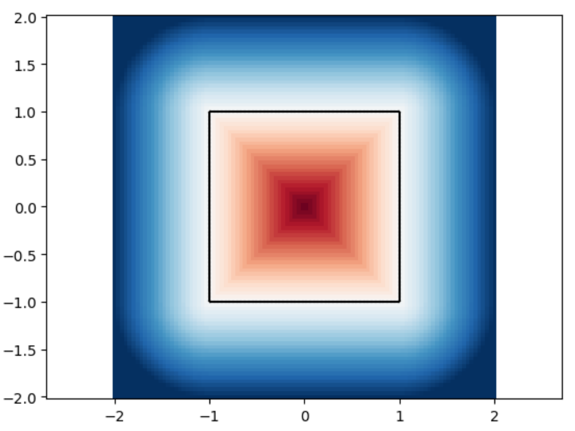
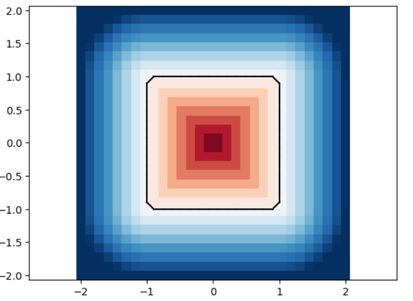
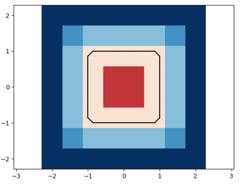
Below are one experiment we did for computing using this inherent error function, the unsquared one. We let the circle sdf be fixed and let the square sdf “escape” from the circle in a constant speed of \(0.2\). That is, we used the union of a fixed circle and a square with changing position as a series of shapes to do analysis. We then draw with color map used in this repo for the ground truths and the marching square results using the common color map.
The inherent error of each union After several trials, one simple observation drawn from this escapaing motion is that when two shapes are more confounding with each other, as in the initial stage, the error is higher; and when the image starts to have two separated connected components, the error rises again. The first one can perhaps be explained by what the paper pointed out as pseudo-sdfs, and the second one is perhaps due to occurence of multipal components.
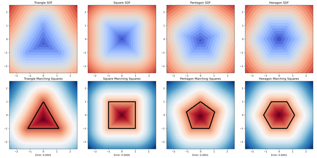
Here is another experiment. We want to know how well this method can simulate the physical characteristics of an object’s rugged level. We used a series of regular polygons. Although the result is theoretically unintheresting as the errors are all nearly zero, this is visually conformting.
Primary mentors: Silvia Sellán, University of Toronto and Oded Stein, University of Southern California
Volunteer assistant: Andrew Rodriguez
Fellows: Johan Azambou, Megan Grosse, Eleanor Wiesler, Anthony Hong, Artur, Sara
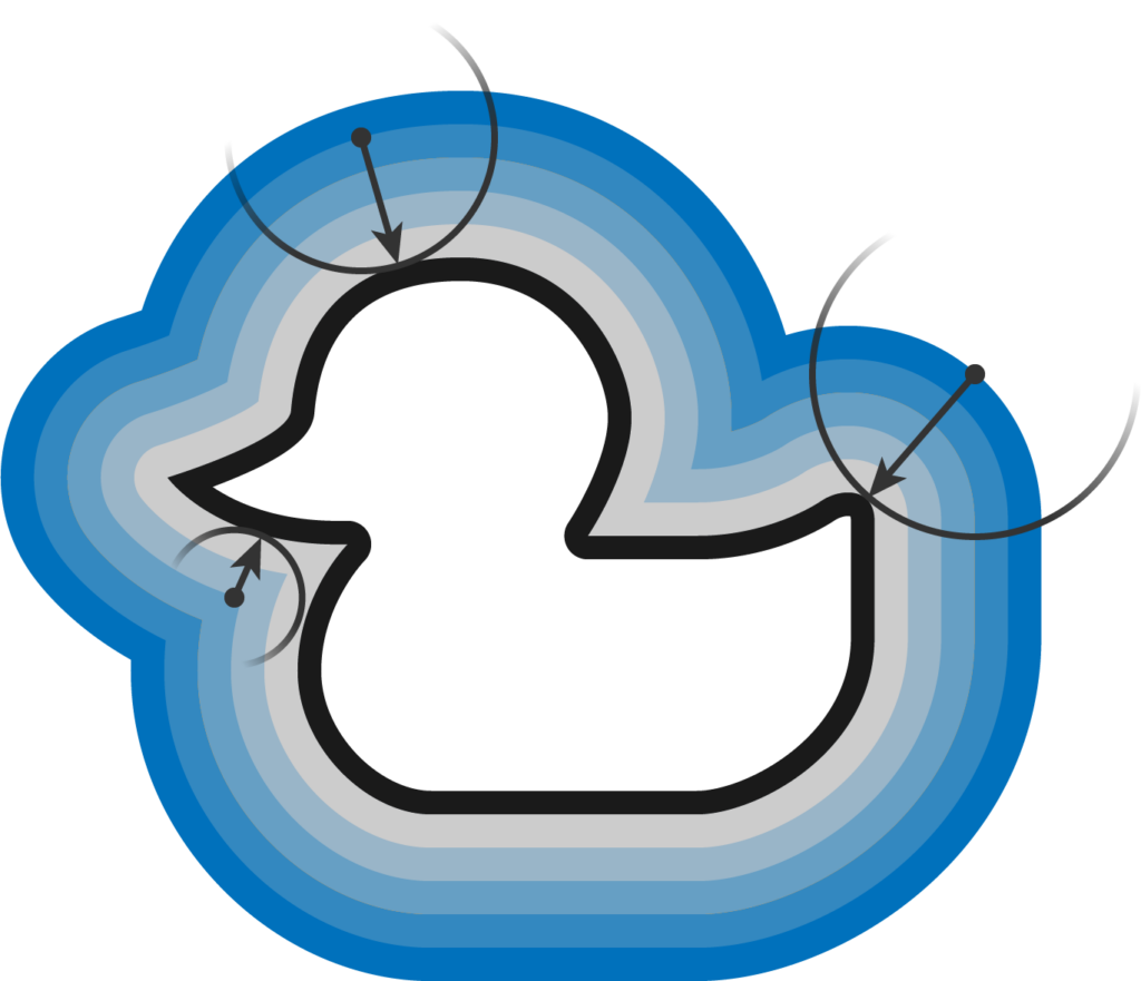
The definition of SDFs using ducks
Suppose that you took a piece of metal wire, twisted into some shape you like, let’s make it a flat duck, and then put it on a little pond. The splash of water made by said wire would propagate as a wave all across the pond, inside and outside the wire. If the speed of the wave were \(1 m/s \), you’d have, at every instant, a wavefront telling you exactly how far away a given point is from the wire.
This is the principle behind a distance field, a scalar valued field \( d(\mathbf{x}) \) whose value at any given point \(\mathbf{x}\) is given by\( d(\mathbf{x}, S) = \min_{\mathbf{y}}d(\mathbf{x}, \mathbf{y})\), where \( S \)is a simpled closed curve. To make this a signed distance field, we can distinguish between the interior and exterior of the shape by adding a minus sign in the interior region.
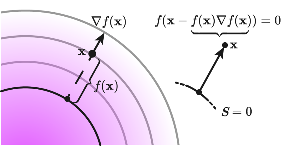
Suppose we were to define sdf without knowing the boundary \(S\); given a region \( \Omega \) and a surface \( S \), whose inside is defined as the closure of \( \overline{\Omega} = A \). A function \( f : \mathbb{R}^n \rightarrow \mathbb{R} \) is said to be a signed distance function if for every point \( \mathbf{x} \in \Omega \) , we have eikonality \( | \nabla f | = 1 \) and closest point condition: \[ f( \mathbf{x} – f(\mathbf{x}) \nabla f(\mathbf{x})) = 0 \]
The statement reads very simply: if we have a point \( \mathbf{x} \), and take the difference vector to the normal of the level set at hand times the distance, it should take us to the point \( \mathbf{x} \) closest to the zero level set.
This second definition is equivalent to the first one by an observation that eikonality implies \(1\)-Lipschitz property of the function \(f\) and it is also used for the last step of the following derivation: \(\exists q \in S:=f^{-1}(0)\) $$ p-f(p) \nabla f(p)=q \Longrightarrow p-q=f(p) \nabla f(p) \Longrightarrow|p-q|=|f(p)| $$
This combined with \(1\)-Lipschitz property gives a proof of contradiction for characterization of sdf by eikonality and closest point condition.
Our project was focused on the SDF-to-Surface reconstruction methods, which is, given a SDF, how can we make a surface out of it? I’ll first tell you about the much simpler problem, which is Surface-to-SDF.
Our SDFs
To lay the foundation, we started with the 2D case: SDFs in the plane from which we can extract polylines. Before performing any tests, we needed a database of SDFs to work with. We created our SDFs using two different skillsets: art and math.
The first of our SDFs were hand-drawn, using an algorithm that determined the closest perpendicular distance to a drawn image at the number of points in a grid specified by the resolution. This grid of distance values was then converted into a visual representation of these distance values – a two-dimensional SDF. Here are some of our hand-drawn SDFs!
The second of our SDFs were drawn using math! Known as exact SDFs, we determined these distances by splitting the plane into regions with inequalities and many AND/OR statements. Each of these regions was then assigned an individual distance function corresponding to the geometry of that space. Here are some of our exact SDF functions and their extracted polylines!
Exact vs. Drawn
Exact Signed Distance Functions (SDFs) provide precise, mathematically rigorous measurements of the shortest distance from any point to the nearest surface of a shape, derived analytically for simple forms and through more complex calculations for intricate geometries. These are ideal for applications demanding high precision but can be computationally intensive. Conversely, drawn or approximate SDFs are numerically estimated and stored in discretized formats such as grids or textures, offering faster computation at the cost of exact accuracy. These are typically used in digital graphics and real-time applications where speed is crucial and minor inaccuracies in distance measurements are acceptable. The choice between them depends on the specific requirements of precision versus performance in the application.
Operations on SDFs
For two SDFs, \(f_1(x)\) and \(f_2(x)\), representing two shapes, we can define the following operations from constructive geometry:
We used these operations to create the following new sdfs: a cat and a tessellation by hexagons.
Marching Squares Reconstructions with Multiple Resolutions
The marching_squares algorithm is a contouring method used to extract contour lines (isocontours) or curves from a two-dimensional scalar field (grid). It’s the 2D analogue of the 3D Marching Cubes algorithm, widely used for surface reconstruction in volumetric data. When applied to Signed Distance Functions (SDFs), marching_squares provides a way to visualize the zero level set (the exact boundary) of the function, which represents the shape defined by the SDF. Below are visualizations of various SDFs which we passed into marching squares with varied resolutions in order to test how well it reconstructs the original shape.
SDF / Resolution
100×100
30×30
8×8
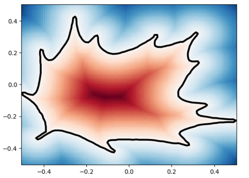
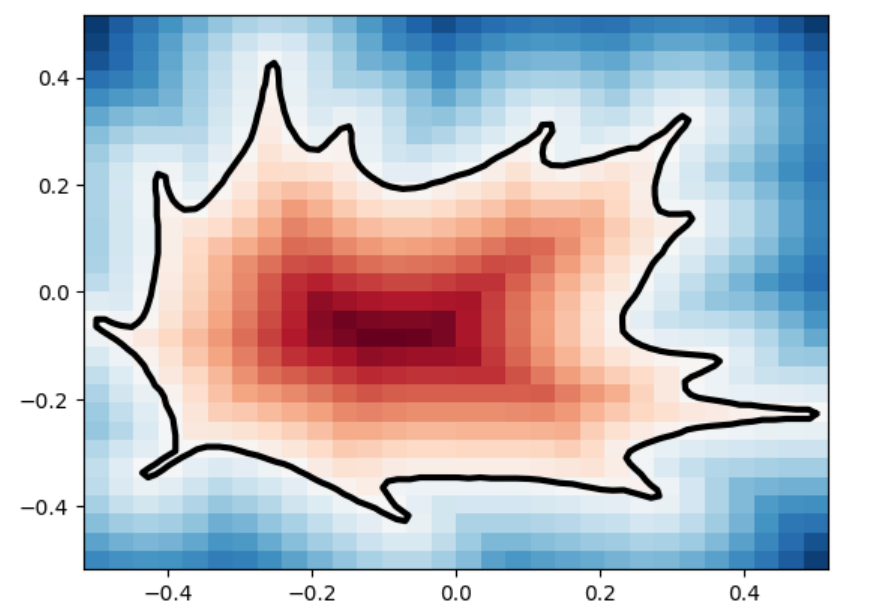
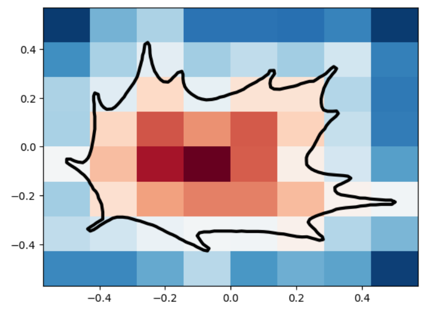
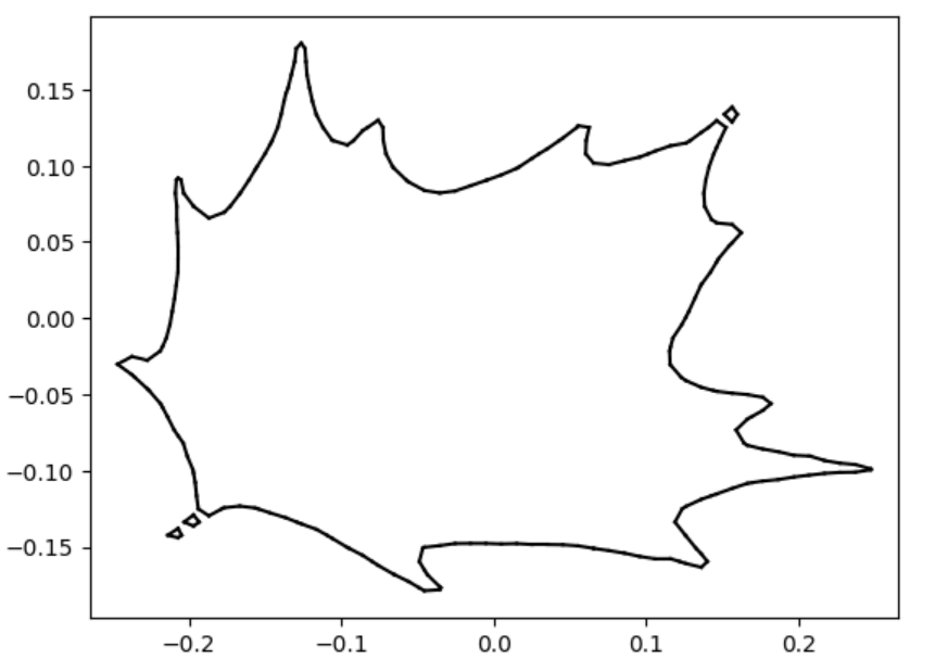
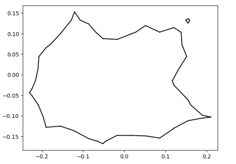
leaf
leaf marching_squares
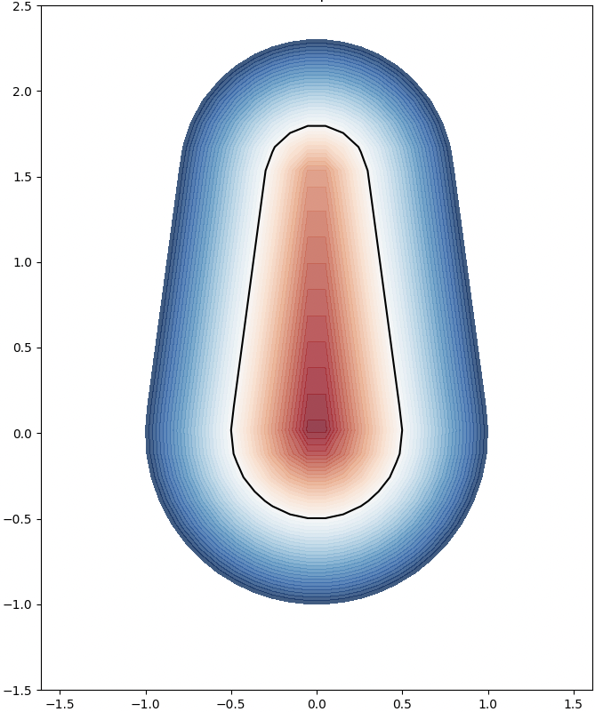
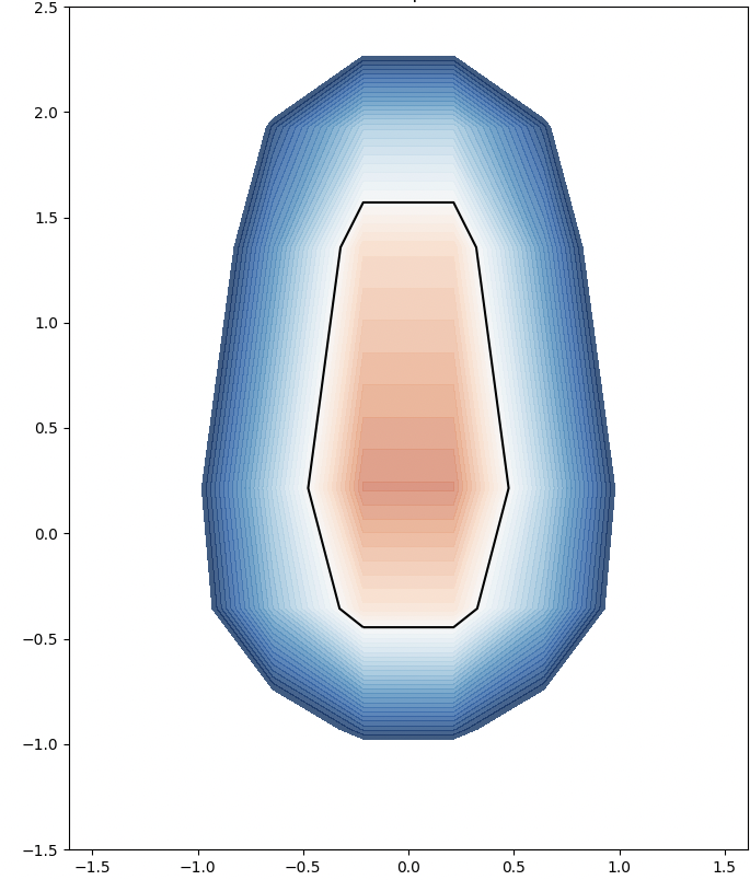
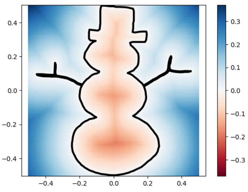
uneven capsule
uneven capsule marching_squares
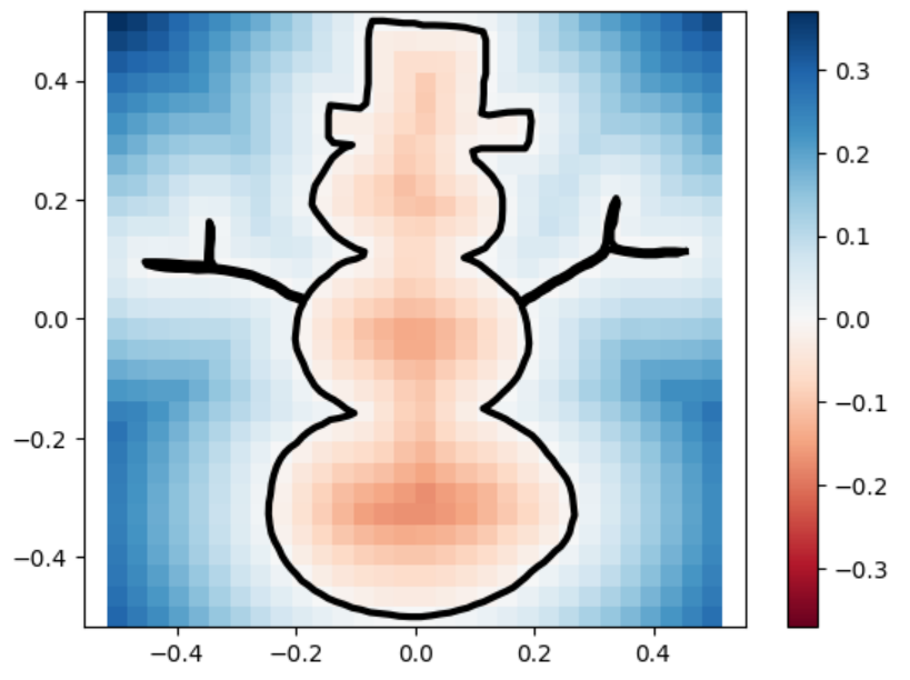
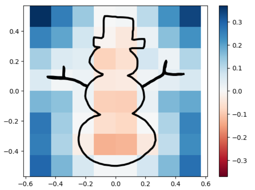
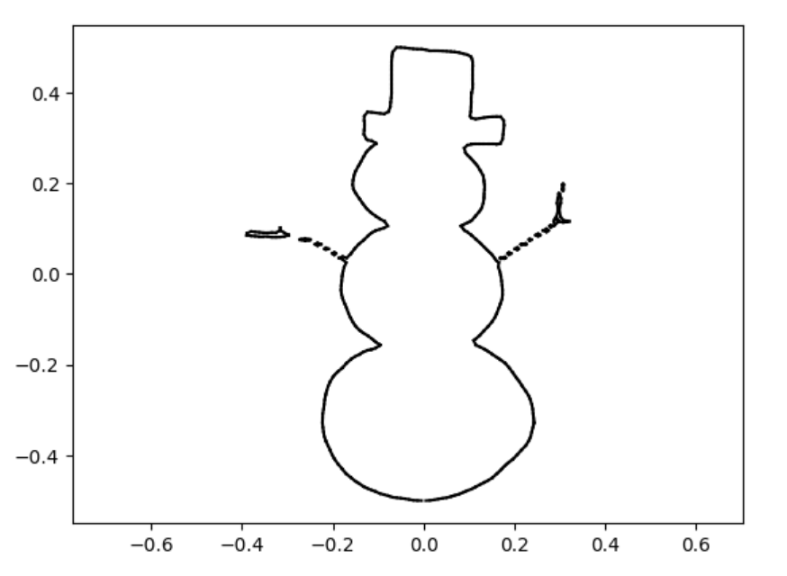
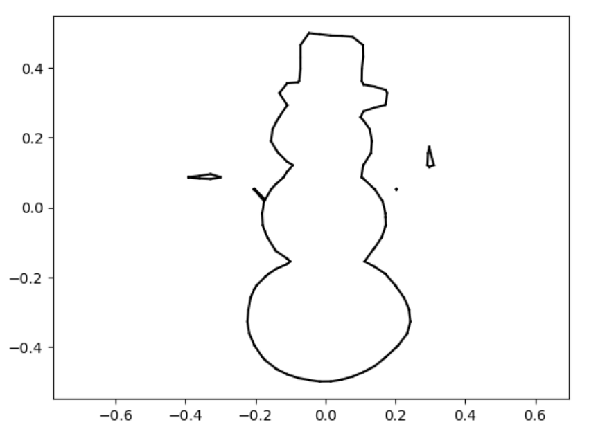
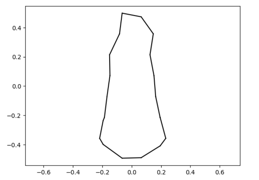
snowman
snowman marching_squares
square
square marching_squares
sdfs and reconstructions in three different resolutions.
SDFs in 3D Geometry Processing
While the work we have done has been 2D in our project, signed-distance functions can be applied to 3D geometry meshes in the same way. Below are various examples from recent papers that use signed distance functions in the 3D setting. Take for example marching cubes, a method for surface reconstruction in volumetric data developed by Lorensen and Cline in 1987 that was originally motivated by medical imaging. If we start with an implicit function, then the marching cubes algorithm works by “marching” over a uniform grid of cubes and then locating the surface of interest by seeing where the surface intersects with the cubes, and adding triangles with each iteration such that a triangle mesh can ultimately be formed via the union of each triangle. A helpful visualization of this algorithm can be found here.
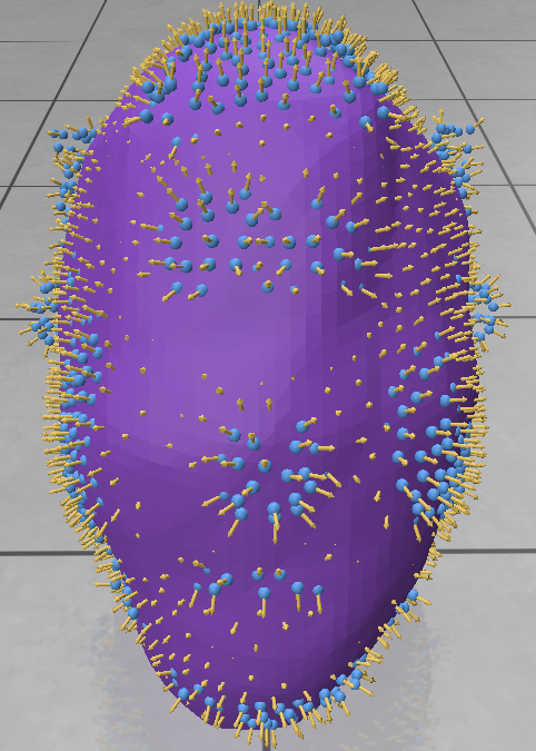
Take for example our mentors Silvia Sellán and Oded Stein’s recent paper “Reach For the Spheres:Tangency-Aware Surface Reconstruction of SDFs” with C. Batty which introduces a new method for reconstructing an explicit triangle mesh surface corresponding to an SDF, an algorithm that uses tangency information to improve reconstructions, and they compare their improved 3D surface reconstructions to marching cubes and an algorithm called Neural Dual Contouring. We can see from their figure below that their SDF and tangency-aware and reconstruction algorithm is more accurate than marching cubes or NDCx.
(From Sellan et al, 2024) The Reach for the Spheres method that using tagency information for more accurate surface reconstructions can be seen on both 10^3 and 50^3 SDF grids as being more accurate than competing methods of marching cubes and NDCx. They used features of SDF and the idea of tangency constraints for this novel algorithm.
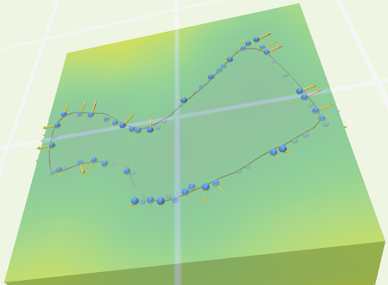
Another SGI mentor, Professor Keenan Crane, also works with signed distance functions. Below you can see in his recent paper “A Heat Method for Generalized Signed Distance” with Nicole Feng, they introduce a novel method for SDF approximation that completes a shape if the geometric structure of interest has a corrupted region like a hole.
(From Feng and Crane, 2024): In this figure, you can see that the inputted curves in magenta are broken, and the new method introduced by Feng and Crane works by computing signed distances from the broken curves, allowing them to ultimately generate an approximated SDF for the corrupted geometry where other methods fail to do this.
Clearly, SDFs are beautiful and extremely useful functions for both 2D and 3D geometry tasks. We hope this introduction to SDFs inspires you to study or apply these functions in your future geometry-related research.
References
Sellán, Silvia, Christopher Batty, and Oded Stein. “Reach For the Spheres: Tangency-aware surface reconstruction of SDFs.” SIGGRAPH Asia 2023 Conference Papers. 2023.
Feng, Nicole, and Keenan Crane. “A Heat Method for Generalized Signed Distance.” ACM Transactions on Graphics (TOG) 43.4 (2024): 1-19.
Marschner, Zoë, et al. “Constructive solid geometry on neural signed distance fields.” SIGGRAPH Asia 2023 Conference Papers. 2023.
Two fundamental mathematical approaches to describing a shape (space) \(M\) involve addressing the following questions:
🤔 (Topological) How many holes are present in \(M\)?
🧐 (Geometrical) What is the curvature of \(M\)?
To address the first question, our space \(M\) is considered solely in terms of its topology without any additional structure. For the second question, however, \(M\) is assumed to be a Riemannian manifold—a smooth manifold equipped with a Riemannian metric, which is an inner product defined at each point. This category includes surfaces as we commonly understand them. This note aims to demystify Riemannian curvature, connecting it to the more familiar concept of curvature.
… Notoriously Difficult…
Riemannian curvature, a formidable name, frequently appears in literatures when digging into geometry. Fields Medalist Cédric Villani in his Optimal Transport said
“it is notoriously difficult, even for specialists, to get some understanding of its meaning.” (p.357)
Riemannian curvature is the father of curvatures we saw in our SGI tutorial and other curvatures. In the most abstract sense, Riemann curvature tensor is defined as a \((0,4)\) tensor field obtained by lowering the contravariant index of the \((1,3)\) tensor field defined as
“It also helps to see pictures of surfaces with zero mean and Gaussian curvature. Zero-curvature surfaces are so well-studied in mathematics that they have special names. Surfaces with zero Gaussian curvature are called developable surfaces because they can be ‘developed’ or flattened out into the plane without any stretching or tearing. For instance, any piece of a cylinder is developable since one of the principal curvatures is zero:” (p.39)
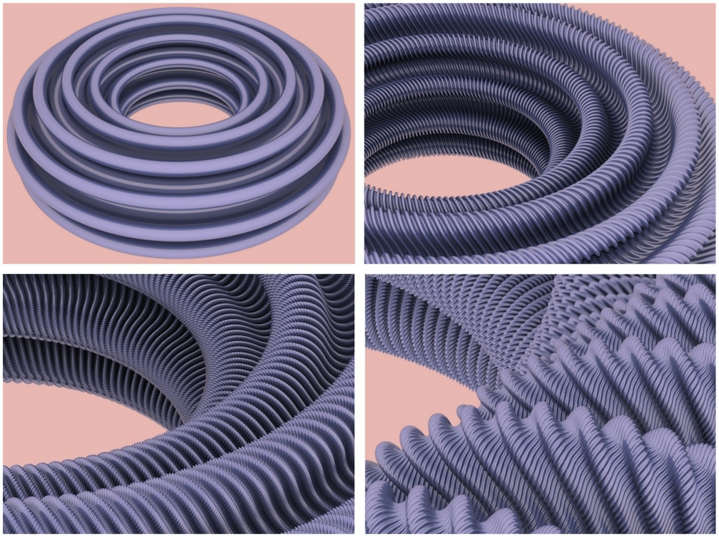
Te following video continues with this cylinder example to show difficulties characterizing flatness. It examines the following question: how to use a piece of flat white paper to roll into a doughnut-shaped object (Torus) without distorting the length of the paper. That is, we are not allowed to use a piece of stretchable rubber to do this job.
This is part of an ongoing project. In fact, in an upcoming SIGGRAPH paper “Repulsive Shells” by Prof. Crane and others, more examples of isometric embeddings, including the flat torus, are discussed.
First definition of flatness
A Riemannian \(n\)-manifold is said to be flat if it is locally isometric to Euclidean space, that is, if every point has a neighborhood that is isometric (distance-preserving) to an open set in \(\mathbb{R}^n\) with its Euclidean metric.
Example: flat torus
We denote the n-dimensional torus as \(\mathbb{T}^n=\mathbb{S}^1\times \cdots\times \mathbb{S}^1\), regarded as the subset of \(\mathbb{R}^{2n}\) defined by \((x^1)^2+(x^2)^2+\cdots+(x^{2n-1})^2+(x^{2n})^2=1\). The smooth covering map \(X: \mathbb{R}^n \rightarrow \mathbb{T}^n\), defined by \(X(u^1,\cdots,u^{n})=(\cos u^1,\sin u^1,\cdots,\cos u^n,\sin u^n)\), restricts to a smooth local parametrization on any sufficiently small open subset of \(\mathbb{R}^n\), and the induced metric is equal to the Euclidean metric in \(\left(u^i\right)\) coordinates, and therefore the induced metric on \(\mathbb{T}^n\) is flat. This is called the Flat torus.
Parallel Transport
We still didn’t answer the question why we need four vector fields to characterize how curved a shape is. We will do this by using another useful tool in differential and discrete geometry to view flatness and thus curvedness. We follow John Lee’s Introduction to Riemannian Manifold for this section, first defining the Euclidean connection.
Consider a smooth curve \(\gamma: I \rightarrow \mathbb{R}^n\), written in standard coordinates as \(\gamma(t)=\left(\gamma^1(t), \ldots, \gamma^n(t)\right)\). Recall from calculus that its velocity is given by \(\gamma'(t)=(\dot{\gamma}^1(t),\cdots,\dot{\gamma}^n(t))\) and its acceleration is given by \(\gamma”(t)=(\ddot{\gamma}^1(t),\cdots,\ddot{\gamma}^n(t))\). A curve \(\gamma\) in \(\mathbb{R}^n\) is a straight line if and only if \(\gamma^{\prime \prime}(t) \equiv 0\). Directional derivatives of scalar-valued functions are well understood in our calculus class. Analogs for vector-valued functions, or vector fields, on \(\mathbb{R}^n\) can be computed using ordinary directional derivatives of component functions in standard coordinates. Given a vector \(v\) tangent to \(M\), we define the Euclidean directional derivative of vector field \(Y\) in the direction \(v\) by:
where for each \(i\), \(v(Y^i)\) is the result of applying the vector \(v\) to the function \(Y^i\): $$ v(Y^i) = v^1 \frac{\partial Y^i(p)}{\partial x^1} + \cdots + v^n \frac{\partial Y^i(p)}{\partial x^n}. $$
If \(X\) is another vector field on \(\mathbb{R}^n\), we obtain a new vector field \(\bar{\nabla} _X Y\) by evaluating \(\bar{\nabla} _{X_p} Y\) at each point: $$ \bar{\nabla}_X Y = X(Y^1) \frac{\partial}{\partial x^1} + \cdots + X(Y^n) \frac{\partial}{\partial x^n}. $$
This formula defines the Euclidean connection, generalizing the concept of directional derivatives to vector fields. This notion can be generalized to more abstract connections on \(M\). When we say we parallel transport a tangent vector \(v\) along a curve \(\gamma\), we simply mean picking vectors for each point on the curve that are tagent to the curve and are parallel to each other at the same time. The mathematical way of saying vectors are parallel is to say the derivative of the vector field formed by them are zero (we have just defined the derivatives for vector field above). Let \(T_pM\) denote the set of all vectors tangent to \(M\) at point \(p\), which forms a vector space.
Given a Riemannian 2-manifold \(M\), here is one way to attempt to construct a parallel extension of a vector \(z \in T_p M\): working in any smooth local coordinates \(\left(x^1, x^2\right)\) centered at \(p\), first parallel transport \(z\) along the \(x^1\)-axis, and then parallel transport the resulting vectors along the coordinate lines parallel to the \(x^2\)-axis.
The result is a vector field \(Z\) that, by construction, is parallel along every \(x^2\) coordinate line and along the \(x^1\)-axis. The question is whether this vector field is parallel along \(x^1\)-coordinate lines other than the \(x^1\)-axis, or in other words, whether \(\nabla_{\partial_1} Z \equiv 0\). Observe that \(\nabla_{\partial_1} Z\) vanishes when \(x^2=0\). If we could show that $$ (*):\qquad \nabla_{\partial_2} \nabla_{\partial_1} Z=0 $$ then it would follow that \(\nabla_{\partial_1} Z \equiv 0\), because the zero vector field is the unique parallel transport of zero along the \(x^2\)-curves. If we knew that $$ (**):\qquad \nabla_{\partial_2} \nabla_{\partial_1} Z=\nabla_{\partial_1} \nabla_{\partial_2} Z,\text{ or } \nabla_{\partial_2} \nabla_{\partial_1} Z-\nabla_{\partial_1} \nabla_{\partial_2} Z = 0 $$ then \((\star)\) would follow immediately, because \(\nabla_{\partial_2} Z=0\) everywhere by construction. We left showing it is true for $\bar{\nabla}$ as an exercise to readers [Hint: use our definition of Euclidean connection above and the calculus fact that \(\partial_{xy}=\partial_{yx}\)]. However, \((**)\) is not generally true for any connection. Lurking behind this noncommutativity is the fact that the sphere is “curved.”
For general vector fields \(X\), \(Y\), and \(Z\), we can study \((**)\) as well. In fact, for \(\bar{\nabla}\), computations easily lead to
and similarly \(\bar{\nabla}_Y \bar{\nabla}_X Z=Y X\left(Z^k\right) \partial_k\). The difference between these two expressions is \(\left(X Y\left(Z^k\right)-Y X\left(Z^k\right)\right) \partial_k=\bar{\nabla}{[X, Y]} Z\). Therefore, the following relation holds for \(\nabla=\bar{\nabla}\): $$ \nabla_X \nabla_Y Z-\nabla_Y \nabla_X Z=\nabla_{[X, Y]} Z . $$
This condition is called flatness criterion.
Second definition of flatness
It can be shown that manifold \(M\) is flat if and only if it satisfies flatness criterion! See Theorem 7.10 of Lee’s.
And finally, we comes back to our definition of Riemannian curvature \(R\) we gave in the first section, which uses the difference between left-hand-side and right-hand-side of above condition to model the deviation of this flatness:
$$ R(X,Y)Z=\nabla_X \nabla_Y Z-\nabla_Y \nabla_X Z-\nabla_{[X, Y]} Z $$
In our deformed mesh project, Dr. Nicholas Sharp showed a cool image of discrete parallel transport in his work with Yousuf Soliman and Keenan Crane.
Some “Downsides”
Now, four is good in the sense that it measures deviation from flatness, but it’s still computationally challenging to understand quantitatively. Besides, the Riemannian curvature tensor provides a lot of redundant information: there are a lot of symmetries of components of \(Rm\), namely, the coefficients \(R_{ijkl}\) such that
These symmetries show that knowing some of them allows to get many of the other components. They are good in that taking a glimpse at some of components gets us a full picture, but they are also bad in that these symmetries indicate that there is redundant information encoded in that tensor field.
Preview: The following will be a brief review on some of the common notions of curvature, since understanding of some of them requires a solid base in Tensor algebra.
We seek to use simpler tensor fields to describe curvature. A natural way of doing this is to consider the trace of the Riemannian curvature. We recall from our linear algebra course that the trace of a linear operator \(A\) is the sum of the diagonal elements of its matrix. This concept can be generalized to trace of tensor products, which can be thought of as the sum of diagonal elements of higher-dimensional matrix of tensor products. Ricci curvature \(Rc\) is the trace of \(Rm=R^\flat\) and scalar curvature \(S\) is the trace of \(Rc\).
Thanks to professor Oded Stein, we already learned in our first week SGI tutorial about principal curvature, mean curvature, and Gaussian curvature. Principal curvatures are the largest and smallest plane curve curvatures \(\kappa_1,\kappa_2\) where curves are intersections of a surface and planes aligning with the (outward-pointing) normal vector at point \(p\). This can be generalized to high-dimensional manifolds by observing that the argmin and argmax happen to be eigenvalues of shape operator \(s\) and the fact that \(h(v,v)=\langle sv,v\rangle\) and \(|h(v,v)|\) is the curvature of a curve, where \(h\) is the scalar second fundamental form. Mean curvature is simply the arithmetic mean of eigenvalues of \(s\), namely \(\frac{1}{2}(\kappa_1+\kappa_2)\) in the surface case; Gaussian curvature is the determinant of matrix of \(s\), namely \(\kappa_1\kappa_2\) in the surface case.
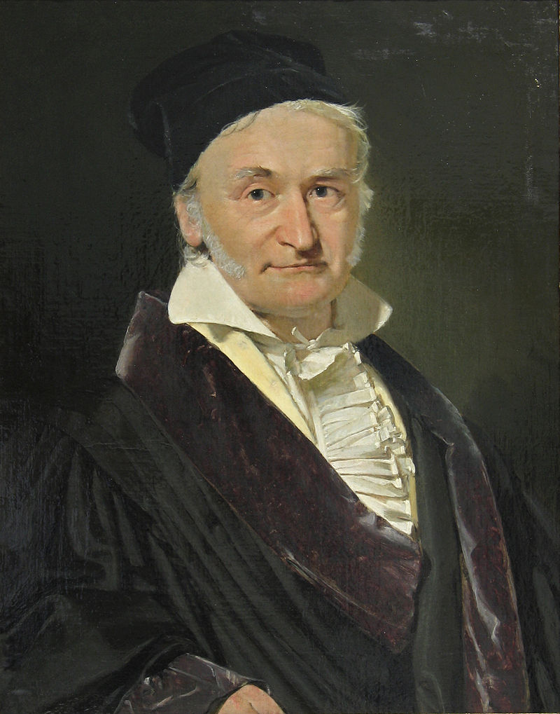
It turns out that Gaussian curvature is the bridge between those abstract Riemannian family \(R,Rm, Rc, S\) and above curvatures that are more familiar to us. Gauss was so glad for finding that Gaussian curvature is a local isometry invariant that he named this discovery as Theorema Egregium, Latin for “Remarkable Theorem.” By this theorem, we can talk about Gaussian curvature of a manifold without worrying about where it is embedded. See here for a demo of Gauss map, which is used for his original definition of Gaussian curvature and the proof of the Theorema Egregium (see here for example). This theorem allows us to define the last curvature notion we’ll used: for a given two-dimensional plane \(\Pi\) spanned by vectors \(u,v\in T_pM\), the sectional curvature is defined as the Gaussian curvature of the \(2\)-dimensional submanifold \(S_{\Pi} = \exp_p(\Pi\cap V)\) where \(\exp_p\) is the exponential map and \(V\) is the star-shaped subset of \(T_pM\) for which \(\exp_p\) restricts ot a diffeomorphism.
Geometric Interpretation of Ricci and Scalar Curvatures (Proposition 8.32 of Lee’s):
My attempt to visualize sectional curvatures.
Let \((M, g)\) be a Riemannian \(n\)-manifold and \(p \in M\). Then
For every unit vector \(v \in T_p M\), \(Rc_p(v, v)\) is the sum of the sectional curvatures of the 2-planes spanned by \(\left(v, b_2\right), \ldots, \left(v, b_n\right)\), where \(\left(b_1, \ldots, b_n\right)\) is any orthonormal basis for \(T_p M\) with \(b_1 = v\).
The scalar curvature at \(p\) is the sum of all sectional curvatures of the 2-planes spanned by ordered pairs of distinct basis vectors in any orthonormal basis.
General Relativity
Writing: Artur RB Boyago
Introduction: Artur studied physics before studying electrical engineering. Although curvatures of two dimensional objects are much easier to describe, physicists still need higher dimensional analogs to decipher spacetime.
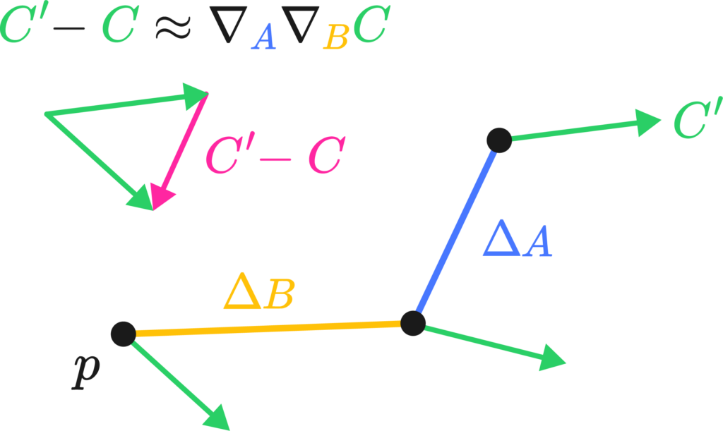
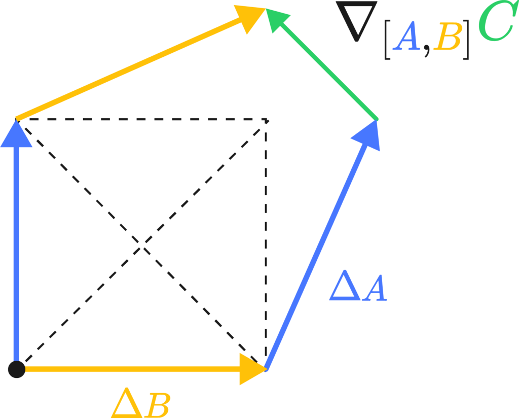
I’d like to give a physicist’s perspective on this whole curvature thing, meaning I’ll flail my hands a lot. The best way I’ve come to understand Riemannian curvature is by the “area/angle deficit” approach. Imagine we had a little bit of a loop made up of two legs, \(\Delta A\) and \( \Delta B\) at a starting point \(p\). Were you to transport a little vector \(C\) down these legs, keeping it as “straight as possible” in curved space. By the end of the two little legs, the vector \( C’ \) would have the same length but a slight rotation in comparison to \(C\). We could, in fact, measure it by taking their difference vector (see the image on the left).
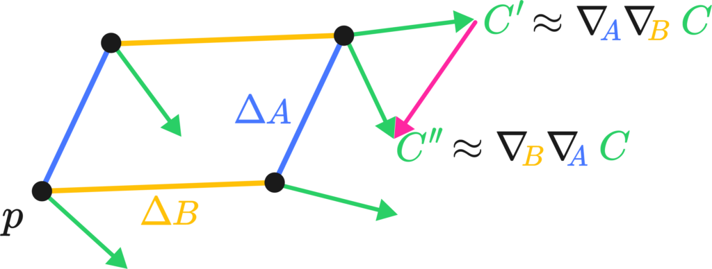
The difference vector is sort of the differential, or the change of the vector along the total path, which we may write down as \( \nabla_A \nabla_B C\), the two covariant derivatives applied to C along \(A\) and \(B\). The critical bit of insight is that changing the order of the transport along \(A\) and \(B\) actually changes the result of said transport. That is, by walking north and then east, and walking east and then north, you end up at the same spot but with a different orientation.
Torsion’s the same deal, but by walking north and then east, and walking east and then north you actually land in a different country.
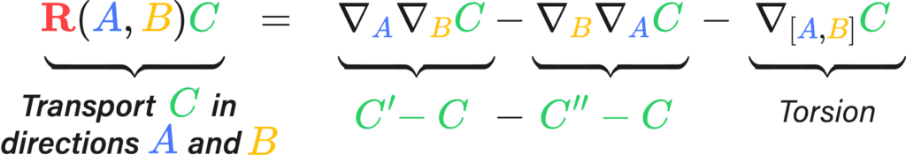
The Riemann tensor is then actually a fairly simple creature. It has four different instructions in its indices, \(R_{abc}^{\sigma}\), and from the two pictures above we get three of them: Riemann measures the angle deficit or the degree of path-dependance of a region of space. This is the \(R_{abc}\) bit
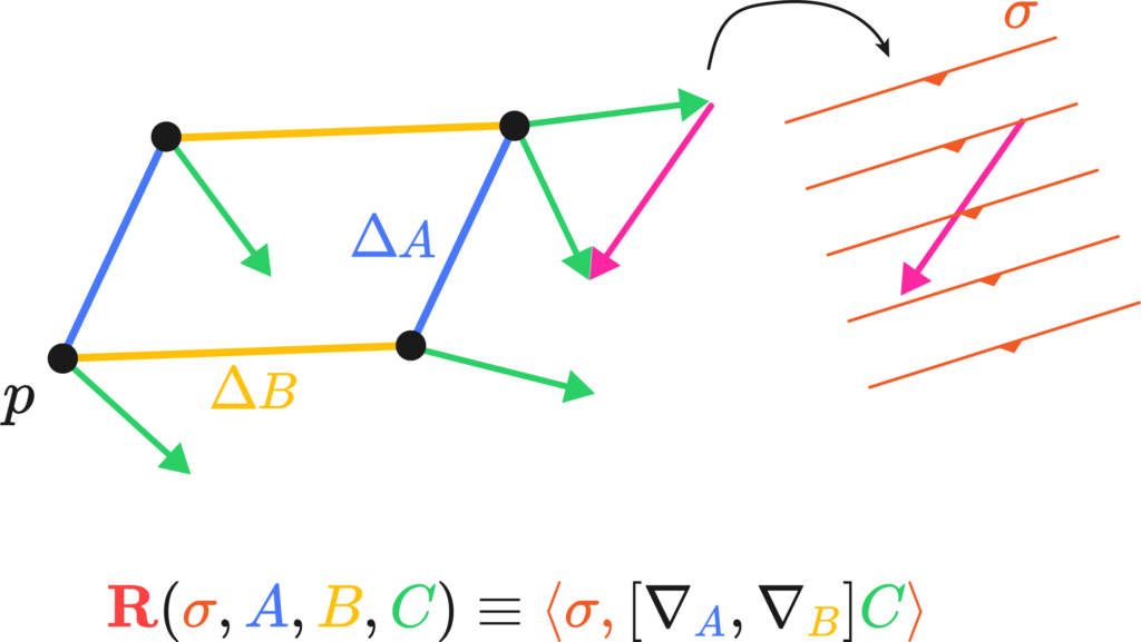
There’s one instruction left. It simply states in which direction we can measure the total difference vector produced by the path by means of a differential form, this closes up our \( R^{\sigma}{abc} \):
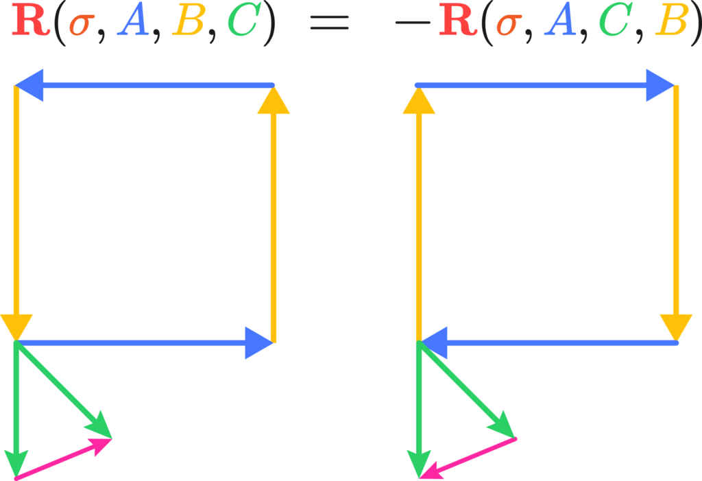
Funny how that works with electrons, they get all confused and get some charge out of frustration. Anyways, the properties of the Riemann tensor can be algebraically understood as these properties of “non-commutative transport” along paths in curved space. For example, the last two indices are naturally anticommutative, since it means the reversal of the direction of travel.
Similarly, it’s quite trivial that by switching the vector being transported and the covector doing the measuring also switches signs: \(R^b_{acd} = -R^a_{bcd}, \; R^a_{bcd} = R^c_{dab}\) The Bianchi Identity is also a statement about what closes and what doesn’t, you can try drawing one that one pretty easily. Now for the general relativity, this is quick; the Einstein tensor is the double dual of the Riemann tensor. It’s hard to see this in tensor calculus, but in geometric algebra it’s rather trivial; the Riemann tensor is a bivector to bivector mapping that produces rotation operators proportional to curvature, the Einstein tensor is a trivector to trivector volume that produces torque curvature operators proportionally to momentum-energy, or momenergy. Torque curvature is an important quantity. The total amount of curvature for the Riemann tensor always vanishes because of some geometry, so if you tried to solve an equation for movement in spacetime you’d be out of luck. But, you can look at the rotational deformation of a volume of space and how much it shrinks proportionally in some section of 3D space. The trick is, this rotational deformation is exactly equal to the content of momentum-energy, or momenergy, of the section. \[\text{(Moment of rotation)} = (e_a\wedge e_b \wedge e_c) \ R^{bc}_{ef} \ (dx_d\wedge dx_e\wedge dx_f) \approx 8\pi (\text{Momentum-energy})\] This is usually written down as\[ \mathbf{G=8\pi T} \]Easy, ay?