Categories
Research

Neural shape sweeping with signed distance functions

Figure 1: Our example 3D implementations of Gpytoolbox sweeping of Stanford bunny and Spot cow object across zig-zag trajectory

By Juan Parra, Kimberly Herrera, and Eleanor Wiesler

Project mentors: Silvia Sellán, Noam Aigerman

Introduction

Given a surface we can represent it moving along certain trajectory in space by a swept area or swept volume. It’s a good idea to take this approach to model 3D shapes or to detect a collision of the shape with another shape in its environment. There are several algorithms in the literature that address the construction of the surface of a swept volume in space, each taking their respective assumptions on the surface and the trajectory.

In our project we trained neural networks to predict the sweeping of a surface, and attempted to find the best representation of a neural network that deals with discontinuities that appear in the process.

Using Signed-Distance Functions to Model Shape Sweeping

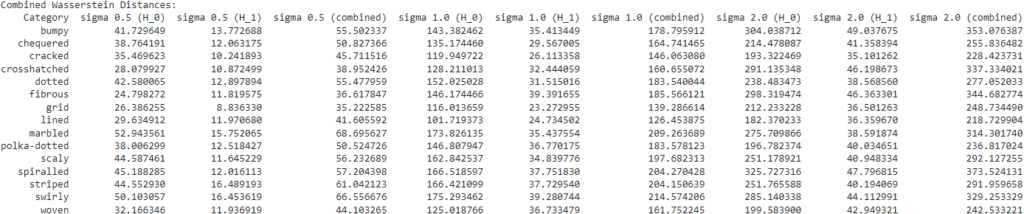
By a swept volume we mean the trajectory that a solid moving through space made. The importance of representing a swept volume can go from art modeling to collision detection in robotics. We can model the swept volume of the solid motion as a surface in 3D. The goal of this project is to train neural networks to learn swept volumes, and so we conducted the experiments of this study using 2D shapes swept across a trajectory in the coordinate plane and evaluated resulting swept area. To study the trajectory or “sweeping” of these shapes, we used Signed Distance Functions (SDFs).

A signed distance function is a way to represent a closed orientable surface S in 3D (or a closed curve in 2D). This signed distance function (SDF) is given by a function: \( D:\mathbb{R}^3\to\mathbb{R} \) such that \( |D(p)| = \min\{d(p,q)^2: q\in S\} \), and the sign of \( D(p) \) is negative if \( p \) is inside the surface and positive otherwise. The zero level set \( D^{-1}(0) \) is equal to the surface \( S \). Given a signed distance function, we can use the Marching Cubes algorithm to construct a mesh representation of the surface. For example, \( G(x,y)=x^2 + y^2 -1 \) is the SDF of the unit circle.
Single circle

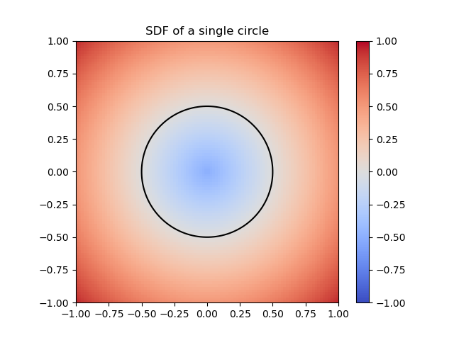
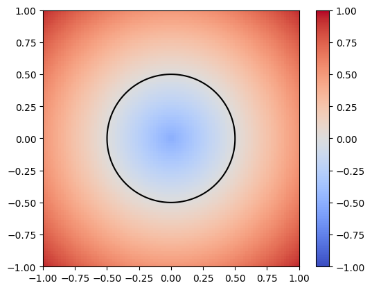
Figure 1: SDF of a single circle

How to represent the SDF of the swept volume of a solid moving through space? We can leverage the operations between SDF’s to construct more complicated surfaces. For instance, the SDF of a unit circle is given by the function \( G(x,y) = x^2 + y^2 – 1 \) and the SDF of a translated circle to the right is \( H(x,y) = (x-0.75)^2 + y^2 – 1 \). So if we wanted to paste both circles as if they were bubbles, we could define the union SDF as: \[ \mathrm{union}(x,y) = \min\{ G(x,y), H(x,y) \} \]
SDF of a union of circles

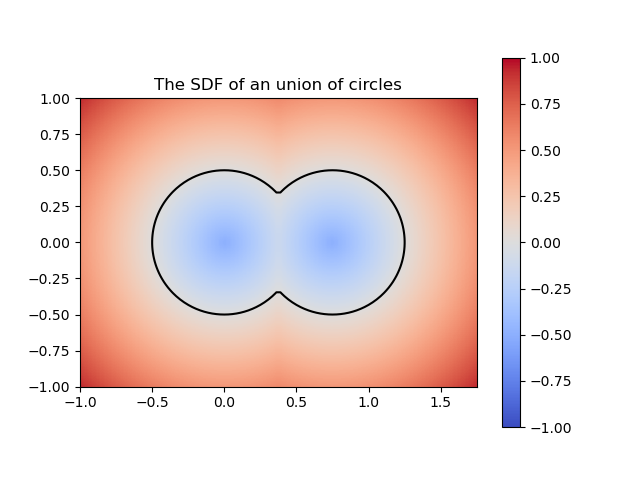
Figure 2: SDF of a union of circles

If we want to perform a continuous motion of the solid we have to model it with a continuous function \(T: [0,1] \to SO(3)\) parametrized by the time, where \(SO(3)\) is the set of rigid motions in 3D (abuse of notation to consider translations as well). Analogously we can think of rigid motions in 2D. Suppose that \(F:\mathbb{R}^3 \to \mathbb{R}\) is the SDF of the solid we’re moving through space with the motion \(T:[0,1] \to SO(3)\). Then the swept volume of the solid is given by the SDF $$ \text{swept volume}(\mathbf{x}) = \min_{t\in[0,1]} F(T_t^{-1}(\mathbf{x})). $$ For the construction of a swept volume (or area) we can start with a previous step, which is to define the function \(t^*:\mathbb{R}^3 \to \mathbb{R}\) $$ t^*(\mathbf{x}) = \mathrm{argmin}_{t\in [0,1]} F(T_t^{-1}(\mathbf{x})), $$ for which we will also have $$ \text{swept volume}(\mathbf{x}) = F \left( T_{t^*(\mathbf{x})}^{-1} (\mathbf{x}) \right). $$ The \(t^*\) function now it’s a “piecewise” continuous function on its domain as shown in the following figures.

Finite Stamping

In order to compute an approximation for the swept volume, one first approach will be to make finite stamping of the SDF moving along a finite discretized sequence of times \(0= t_1< \cdots< t_n=1\) and then compute the SDF $$ \text{swept volume approximation}(\mathbf{x}) = \min_{t\in \{t_1, \ldots, t_n\}} F(T_t^{-1}(\mathbf{x})). $$ For example, if we define an SDF of a bone (see next 3 images), and let's say we defined the motion \(T_t(x,y) = (x,y) + (t, \sin(t))\), then depending on how fine is our discretization, we can have a good or a bad approximation.

(a) 20 times

(b) 100 times

In this case we can also define an approximation to the \(t^*\) function as follows $$ t^*_{\text{approx}}(\textbf{x}) = \text{argmin}_{t \in \{ t_1, \ldots, t_n \}} F(T_{t}^{-1} (\mathbf{x})). $$ However, we can notice that looking for the argument of the minimum of a function can be computationally expensive, and that’s something we may want to do only once in our lifes. Maybe we could substitute our Finite Stamping SDF with a neural network. Knowing that \(t^*\) is not a continuous function, it will be interesting to fit a neural network to it, and play with its architecture so we find a neural network that represents better those discontinuities.

Learning Swept SDFs with Neural Networks

How to use a NN for SDFs

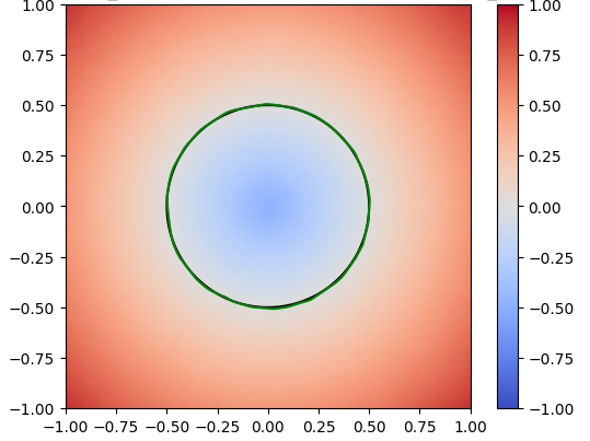
A neural network is just a function with many parameters; we can tweak these parameters to best approximate an SDF. To train the network, we first sample random points from the circle and compute their actual SDF values. The network’s goal is to predict these SDF values. By comparing the predicted values to the actual values using a loss function, the network can adjust its parameters to reduce the error. This adjustment is typically done through gradient descent, which iteratively refines the network’s parameters to minimize the loss. After training, we visualize the results to assess how well the neural network has learned to approximate the SDF. In the image below, the green represents the prediction for the circle by the neural network.

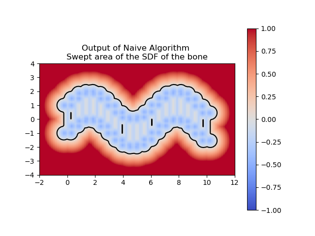
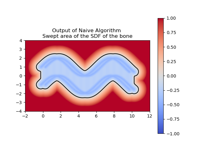
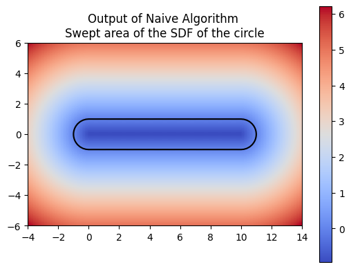
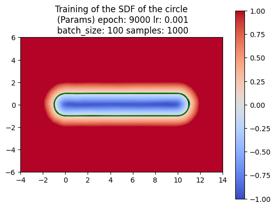
For computing a swept area, the neural network needs to approximate the union of multiple SDFs that together represent the swept area. Computing the swept area involves shifting the SDF along the trajectory at various points in time and then taking the union of all these SDFs. Once we understood how to compute the swept area ourselves, we had the neural network attempt the same. The following images show the results of our manual computation, which we refer to as the naive algorithm, for the sweeping of the circle along a horizontal path in comparison to the computation produced by the neural network. Similarly, the green represents the prediction for the swept area by the neural network.

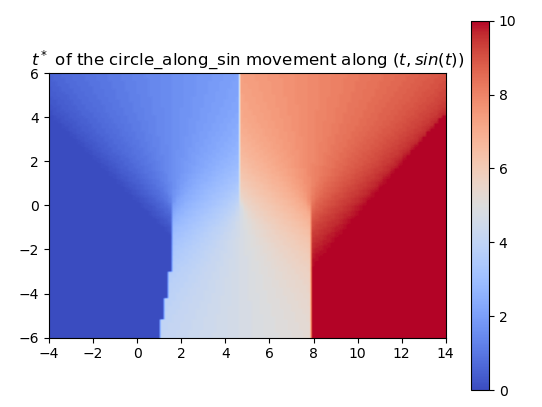
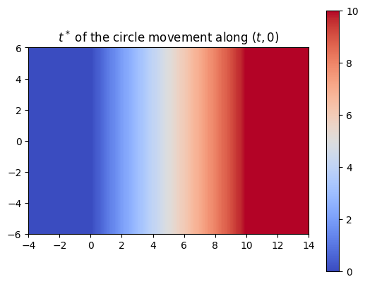
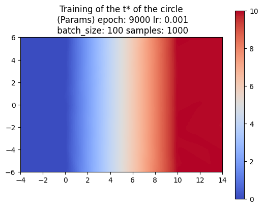
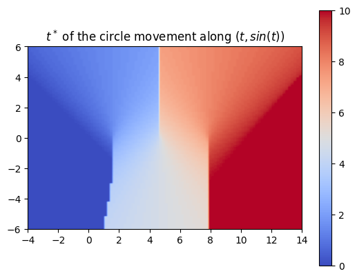
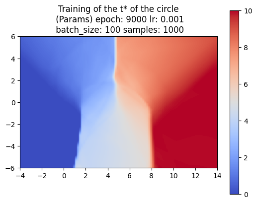
So far, we’ve trained the neural network to compute the SDF values for each point in a 2D grid. Now, since we are sweeping a shape over time, we want the network to return the times corresponding to these SDF values. We call these times t*. With the same shape and trajectory as above, the network has little issue doing this.

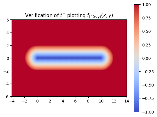
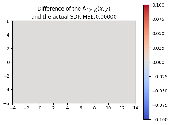
We also made sure that the t*‘s that we computed were producing the correct SDF of the swept area.

NN Difficulties detecting discontinuities

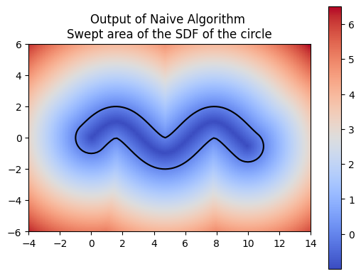
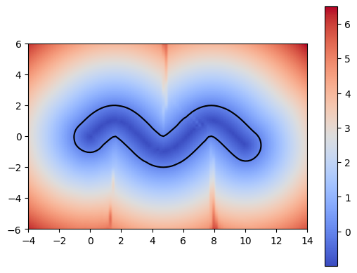
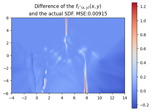
Using a more complex trajectory, such as a sine wave, introduces some challenges. While the neural network performs well in predicting the t* values, issues arise when computing the SDF with respect to these times. Specifically, the resulting SDF shows three lines emerging from the peaks and troughs of the curve. We can see this even more through the MSE plot.

The left image shows the sweeping of the circle using the t* values computed by the neural network.

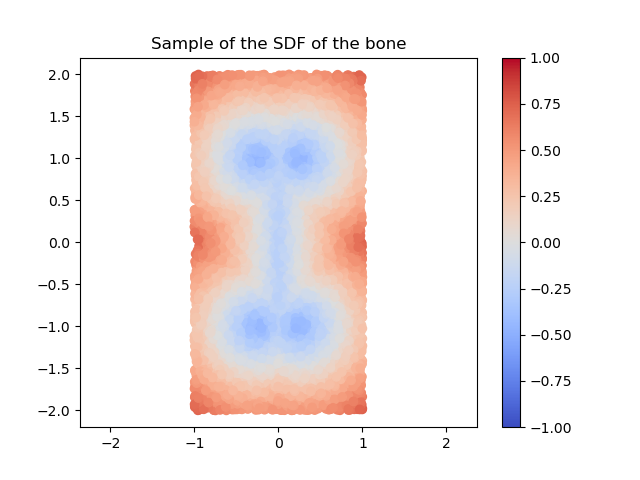
These challenges become even more apparent when using shapes with sharper edges such as a square. Because of this, we decided to work on optimizing the neural network architecture.

Adjusting Our Neural Network Architecture

Changing Our Activation Function

Every neural network has a defined activation function. In the case of our preliminary neural network experiments above, the specified activation function was a Rectified Linear Unit (ReLU). Despite this, we did not achieve the most desirable outcome of minimal error in the predicted swept SDF versus the naive algorithm swept SDF. Specifically, we observed errors at sites of discontinuity, where there were changes in sign, for example.

In an attempt to improve neural network performance, we decided to experiment with different activation functions by altering our neural network architecture. Below, we present their corresponding results when used for swept SDF prediction.

ReLU Function (Rectified Linear Unit Function)

f(x) = { 0 for  x < 0 x for  x ≥ 0

Logistic Sigmoid Function

f(x) = 1 1 + e x

Hyperbolic Tangent Function

f(x) = tanh ( x ) = 2 1 + e 2 x 1

Categories
Uncategorized

Topology of feature spaces

CLIP is a system designed to determine which image matches which piece of text in a group of images and texts.

1. How it works:

• Embedding Space: Think of this as a special place where both images and text are transformed into numbers.

• Encoders: CLIP has two parts that do this transformation:

– Image Encoder: This part looks at images and converts them into a set of numbers (called embeddings).

– Text Encoder: This part reads text and also converts it into a set of numbers(embeddings).

2. Training Process:

• Batch: Imagine you have a bunch of images and their corresponding texts in a group(batch).

• Real Pairs: Within this group, some images and texts actually match (like an image of a cat and the word ”cat”).

• Fake Pairs: There are many more possible combinations that don’t match (like an image of a cat and the word ”dog”).

3. Cosine Similarity: This is a way to measure how close two sets of numbers (embeddings) are. Higher similarity means they are more alike.

4. CLIP’s Goal: CLIP tries to make the embeddings of matching images and text (real pairs) as close as possible. At the same time, it tries to make the embeddings of non-matching pairs (fake pairs) as different as possible.

5. Optimization:

• Loss Function: This is a mathematical way to measure how good or bad the current matchings are.

• Symmetric Cross-Entropy Loss: CLIP uses a specific type of loss function that looks at the similarities of both real and fake pairs and adjusts the embeddings to improve the matchings.

In essence, CLIP learns to accurately match images and texts by continuously improving how it transforms them into numbers so that correct matches are close together and incorrect ones are far apart.

After learning CLIP, I chose my data set and got to work:

The Describable Textures Dataset (DTD) is an evolving collection of textural images in the wild, annotated with a series of human-centric attributes, inspired by the perceptual properties of textures.

The package contains:

1. Dataset images, train, validation, and test.

2. Ground truth annotations and splits used for evaluation.

3. imdb.mat file, containing a struct holding file names and ground truth labels.

Example images:

There are 47 texture classes, with 120 images each for a total of 5640 images in this data set. The above shows ‘cobwebbed’, ‘pitted,’ and ‘banded’. I did the t-SNE visualization by class for all the classes but realized this wasn’t very helpful for analysis. It was the same for UMAP. So I decided to sample 15 classes and then visualize:

In the t-SNE for 15 classes, we see that ’polka-dotted’ and ’dotted’ are clustered together. This intuitively makes sense. To further our analysis, we computed the subspace angles between the classes. Many pairs of categories have an angle of 0.0, meaning their feature vectors are very close to each other in the feature space. This suggests that these textures are highly similar or share similar feature representations. For instance:

• crosshatched and striped

• dotted and grid

• dotted and polka-dotted

Then came the tda: A persistence diagram summarizes the topological features of a data set across multiple scales. It captures the birth and death of features such as connected components, holes, and voids as the scale of observation changes. In a persistence diagram, each feature is represented as a point in a two-dimensional space, where the x-coordinate corresponds to the “birth” scale and the y-coordinate corresponds to the “death” scale. This visualization helps in understanding the shape and structure of the data, allowing for the identification of significant features that persist across various scales while filtering out noise.

I added 3 levels of noise (0.5, 1.0, 2.0) to the images and then extracted features. I visualized these features on a persistence diagram. Here are some examples of those results. We can see that for H_0 at all noise levels, there is one persistent feature so there is one connected component. The death of this persistent feature varies slightly. H_1 at all noise levels there aren’t any highly persistent features, with most points being around the diagonal. The features in H_1 tend to “clump up together” and die quicker as the noise level goes up.

I then computed the distances between the diagrams with no noise and those with noise. Here are some of those results. Unsurprisingly, with greater levels of noise, there is greater distance.

Finally, we wanted to test the robustness of CLIP so we classified images with respect to noise. The goal was to see if the results we saw with respect to the topology of the feature space corresponded to the classification results. These were the classification accuracies:

We hope to discuss our results further!

Categories
Uncategorized

SGI Thus Far

Hello world! I’m Kimberly Herrera. I was born and raised in LA county but I’m currently in the Bay Area where I’m a senior at UC Berkeley. I study pure math and math education. I applied to SGI because I had previously gotten a taste of topological data analysis this previous summer and I guess I wanted to see other ways in which math and coding ‘mesh.’😎

Tutorial week
I’m in California so that meant waking up before 8 am which kinda sucked but I got used to it. I’m also someone who has a hard time learning remotely so I was worried, but thankfully the lecturers were great. I was able to follow along (mostly) while growing interested in the material. I think my favorite lesson was on 2D and 3D shape representations. This wasn’t particularly new to me, having worked with point clouds and cubic splines before, but Silvia was a very engaging speaker. She presented the material in a way that was so digestible. By the end of the week, I hadn’t nearly finished all of the exercises but I made sure to do a few from each lesson so I could be prepared for the coming weeks.


When ranking projects, a lot of the descriptions were just buzzwords for me. I just decided to choose whichever ones had prerequisites I satisfied. I actually got my first choice for my first project, which I chose because it involved tda.

Project 1:
In our first meeting, we introduced ourselves and our background in topology and machine learning. Our mentor then told us the goals of the project, which I made sure to write down. We then immediately went to work. I started by investigating the neural network CLIP we would be using for image classification. I also researched what feature spaces were. This project went on for 2 weeks and we only met as a team like 4 times, although we did consistently communicate through Slack. However, it did feel like “here’s what you need to do, now go do it,” which was fine with me. I was proud of my work on this project, I completed everything I needed to do and was able to communicate my findings in our meetings.

Project 2:
This project is so different from the last. This mentor started by presenting slides on the background and goals for the project. I also noticed that the TA was more active, I think because they are a graduate student of the mentor. We also meet every day in the morning and have a follow-up meeting to discuss our work for the day. That being said, I don’t think I’ve completed as much work on this project thanks to errors with running the code. Hopefully, more progress will be made in the coming days.

In comparison to previous research:
SGI has been a bit different from the REU I did last summer. Having a tutorial week and guest lectures is the same, but here we do multiple mini projects instead of deep diving into one sole project. This of course leads to engaging with different kinds of people and different work ethics. Last summer I was working 9-5 while this time it depends on the project and the mentor. Another big difference of course is how coding/cs heavy this project is compared to my previous project. Previously, we did a deeper dive into the mathematical background (since it was a math REU) and the coding was done to inform the math. Now it feels like the math is learned in order to inform the CS/Machine learning.

Overall, I am having a good time and am excited for the next two weeks 🙂