Categories
Uncategorized

What Are Implicit Neural Representations?

Usually, we use neural networks to model complex and highly non-linear interactions between variables. A prototypical example is distinguishing pictures of cats and dogs.
The dataset consists of many images of cats and dogs, each labelled accordingly, and the goal of the network is to distinguish them in a way that can be generalised to unseen examples.

Two guiding principles when training such systems are underfitting and overfitting.

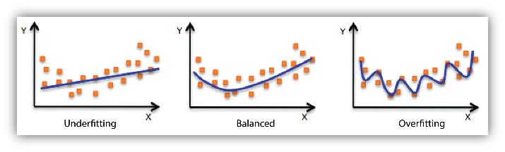
The first one occurs when our model is not “powerful enough” to capture the interaction we are trying to model so the network might struggle to learn even the examples it was exposed to.

The second one occurs when our model is “too powerful” and learns the dataset too well. This then impedes generalisation capabilities, as the model learns to fit exactly, and only, the training examples.

But what if this is a good thing?

Implicit Neural Representations

Now, suppose that you are given a mesh, which we can treat as a signed distance field (SDF), i.e. a function f : R3 \to R, assigning to each point in space its distance to the mesh (with negative values “inside” the mesh and positive “outside”).

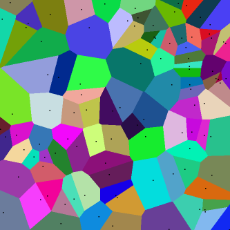
This function is usually given in a discrete way, like a grid of values:

But now that we have a function, the SDF, we can use a neural network to model it to obtain a continuous representation. We can do so by constructing a dataset with input x = (x,y,z) a point in space and label the value of the SDF at that point.

In this setting, overfitting is a good thing! After all, we are not attempting to generalise SDFs to unseen meshes, we really only care about this one single input mesh (for single mesh tasks, of course).

But why do we want that?

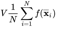
We have now built a continuous representation of the mesh, and we can therefore exploit all the machinery of the continuous world: differentials, integration, and so on.

This continuous compression can also be used for other downstream tasks. For example, it can be fed to other neural networks doing different things, such as image generation, superresolution, video compression, and more.

There are many ways to produce these representations: choice of loss function, architecture, mesh representation…
In the next blog posts, we will discuss how we do implicit neural representations in our project.

Categories
Math

Voronoi Tessellations

Last week, we looked into Voronoi tessellations and their potential for high dimensional sampling and integral approximations.

When we have a very complicated high-dimensional function, it can be very challenging to compute its integral in a given domain. A standard way to approximate it is through Monte Carlo integration

Monte Carlo integration

Monte Carlo integration is a technique consisting of querying the integrand function f at N random locations uniformly, taking the average, and then multiplying the region’s volume:

The law of large numbers ensures that, in the limit, this quantity approximates the actual integral better and better.

Okay, but the points are sampled i.i.d. uniformly, which might not be optimal to compute the integral’s value from a very small sample size. Maybe we can find a way to guide the sampling and leverage prior knowledge we might have about the sample space.
Okay, and maybe the points are not extracted i.i.d. What if we have no control over the function – maybe it’s some very big machine in a distant factory, or an event occurring once in a decade. If we can’t ensure that the points are i.i.d. we just can’t use Monte Carlo integration.

Therefore, we will investigate whether we can use Voronoi tessellations to overcome this limitation.

Voronoi Tessellation

A Voronoi tessellation is a partition of the space according to the following rules:

  • We start with some “pivot” points pi in the space (which could be the points at which we evaluate the integrand function)
  • Now, we create as many regions as there are initial pivot points defined as follows: a point x in the space belongs to the region of the point pi if the point pi is the closest pivotal point to x :

Voronoi tessellation is essentially one iteration of k-means clustering where the centroids are the pivotal points pi and the data to cluster are all the points x in the domain

Some immediate ideas here:

  • We can immediately try out “Voronoi integration”, where we multiply the value of the integrand at each starting point f(pi) by the volume of its corresponding region, summing them all up, and see how it behaves compared to Monte Carlo integration (especially in high dimensions)
  • We can exploit Bayesian optimisation to guide the sampling of the points pi as we don’t require them to be i.i.d. unlike Monte Carlo integration
  • We can exploit prior knowledge on the integration domain to weight the areas by a measure


In the next blog posts, we will see some of these ideas in action!