yixinlok – SGI 2024

Project Mentor: Nicholas Sharp

SGI Volunteer: Qi Zhang

This blog post is a follow up to “How to match the “wiggliness” of two shapes”, where we discussed the metrics we use to measure the similarity between two surfaces. In that post, we briefly talked about approximating a surface by using a regular grid to generate vertices for an approximation mesh. There we observed that as we increased the number of vertices, the surface approximation error decreases. This is somewhat intuitive – as you increase the “fineness” of the approximation mesh, the more closely you would expect it to approximate the actual surface. However, in practical applications we aim to keep the number of vertices as low as possible, in order to reduce both memory space and the amount of runtime computation.

So what can we do to improve the surface approximation without increasing the number of vertices? Are there better ways to select vertices – such that we can minimize the chamfer distance error? This is what we will be exploring in this post.

Regular grids

Before we try different ways of selecting vertex positions. Hence we repeat the same experiment with a few different surfaces, using a regular grid to generate mesh vertices. First we start with three basic cases with different gaussian curvatures:

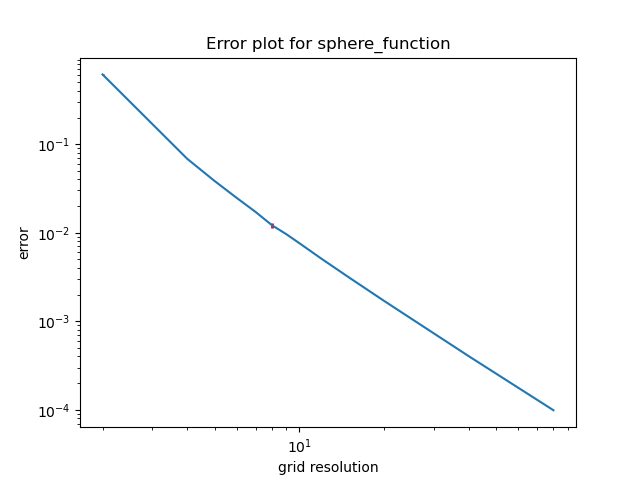
Sphere function (positive gaussian curvature)

Figure 1. Sphere function approximated with regular grid vertices.

Figure 2. Log-log error plot of grid vertices dimensions and chamfer distance error for the sphere function

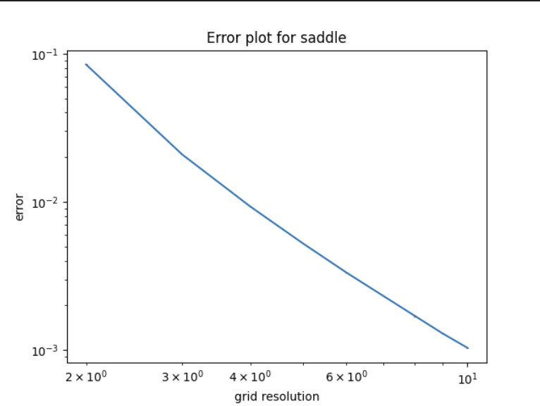
2. Saddle function (negative gaussian curvature)

Figure 3. Saddle function approximated with regular grid vertices.

Figure 4. Log-log error plot of grid vertices dimensions and chamfer distance error for the saddle function

3. Quadratic function (0 gaussian curvature)

Figure 5. Quadratic function approximated with regular grid vertices.

Figure 6. Log-log error plot of grid vertices dimensions and chamfer distance error for the quadratic function

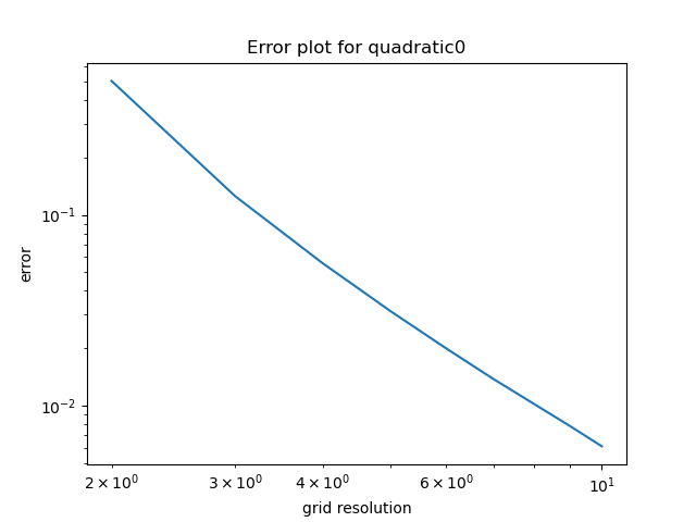
So far everything works well similarly to the previous blog post – the error decreases consistently as the grid resolution.

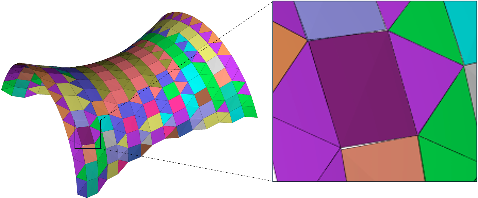
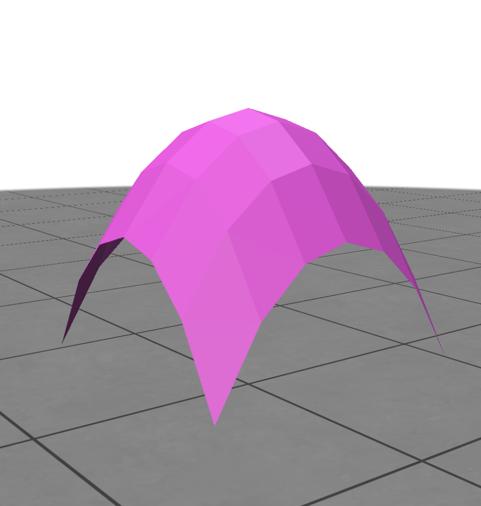
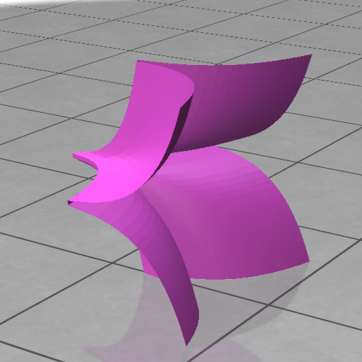
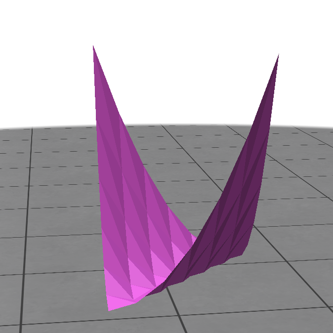
In order to really visualize the limitations of using the regular grid to sample points on the mesh, we decided to also include a more “extreme” function that looks harder to approximate – the Cross-in-tray function, which has a few asymptotes.

4. Cross-in-tray function

Figure 7. Cross-in-tray function approximated with regular grid vertices

For this function, we noticed something unusual. When we increase the grid resolution from 6×6, to 7×7, to 8×8, we notice a sharp increase, then decrease in error, unlike the consistent decrease in error as we saw before.

Figure 8. Error plot of grid vertices dimensions and chamfer distance error for the quadratic function

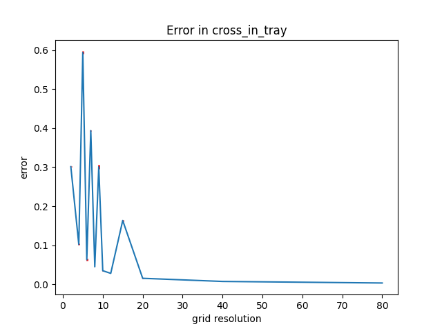
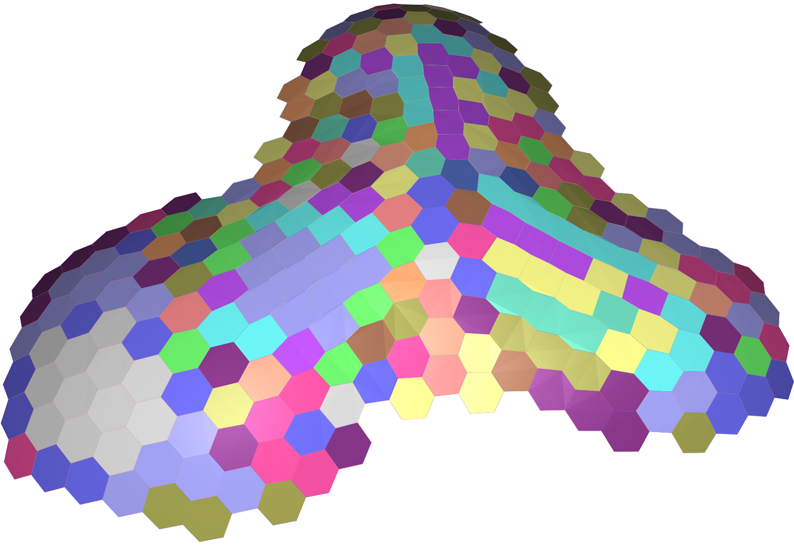
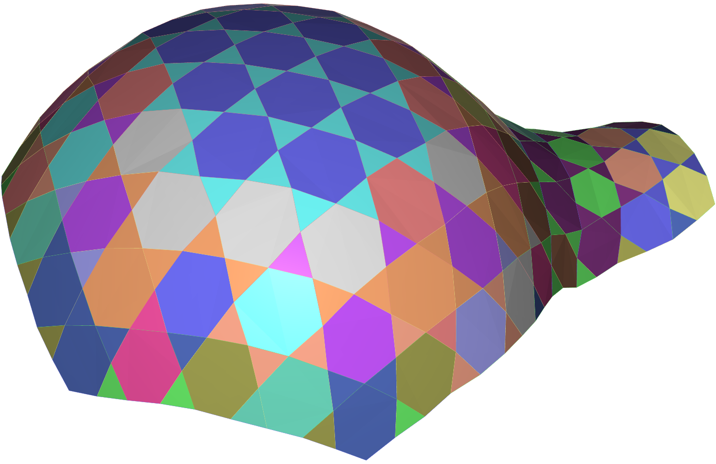
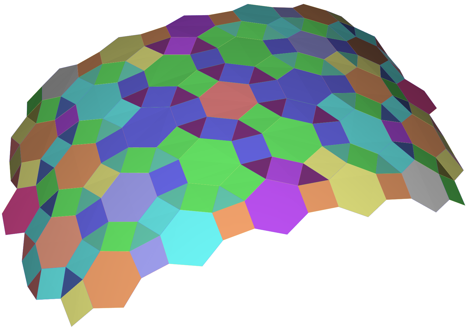
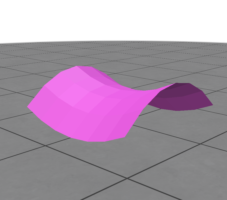
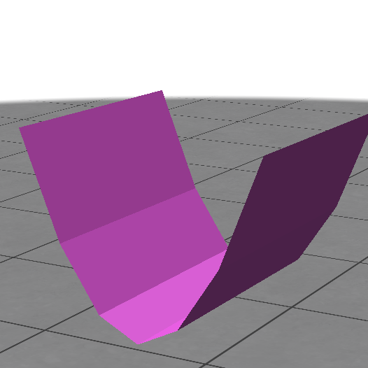
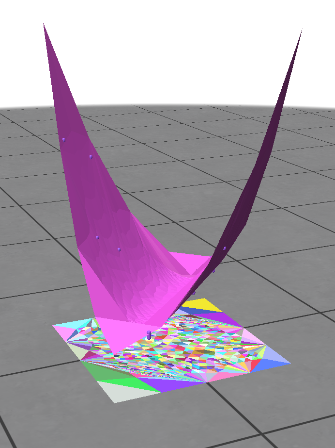
We decided to visualize what might be causing this in the figures 9-11 below, where the green transparent surface represents a close approximation of the actual surface, and the magenta surface shows the surface generated by sampling the regular grids with the different dimensions mentioned .

Figure 9. Approximation with 6×6 grid vertices

Figure 10. Approximation with 7×7 grid vertices

Figure 11. Approximation with 8×8 grid vertices

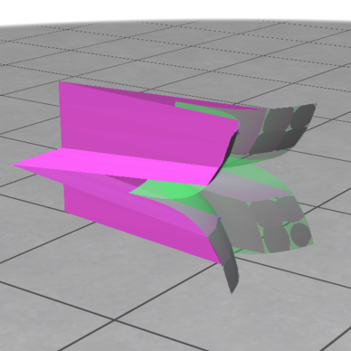
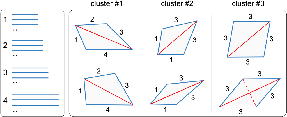
As seem above, the increase in the approximation error for the 7×7 regular grid is caused by the alignment of the selected vertices with the planes that the asymptotes lie on.

This is an interesting observation, as we can visibly see that the alignment of the vertices to certain features or properties of a surface affects the surface approximation error. There have been works [1][2] that have touched on heuristics about how when the mesh edges are orthogonal to the direction of principal curvature of the original function it often (but not always!) results in a lower approximation error. The next two type of experiments look into this further.

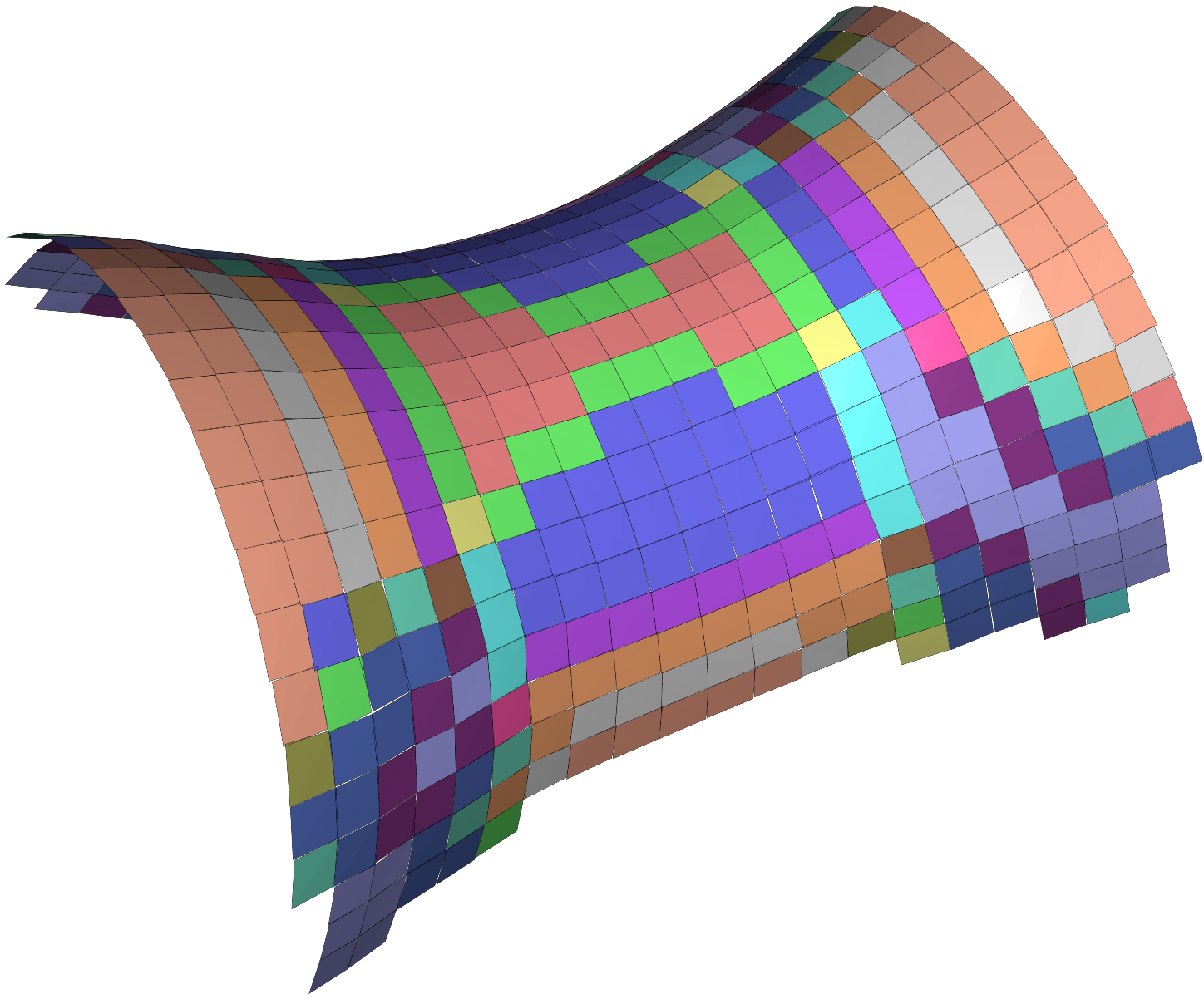
Rotated surface function

We decided to test the alignment of the edges to the direction of principal curvature on the quadratic function, as we could easily identify this direction for this function. We rotated the surface by different angles and generated approximations using the same regular grid, then plotted its error.

Figure 12. Approximation of unrotated quadratic function

Figure 13. Approximation of quadratic function rotated 45 degrees around the z axis

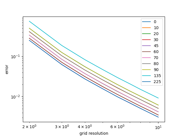
Interestingly, the error is the lowest when the quadratic function is rotated 45 degrees and 225 degrees and highest. This is notable because when the function is rotated 0 or 90 degrees, the short edges of the triangles are in fact orthogonal to the direction of principal curvature, so according to the heuristic these cases should have given the lowest error.

After closer observation we realized that the 45 degrees and 225 degrees cases are when the longest edge of the triangles are orthogonal with the curvature of the quadratic surface. Perhaps more work can be done to look into this in the future!

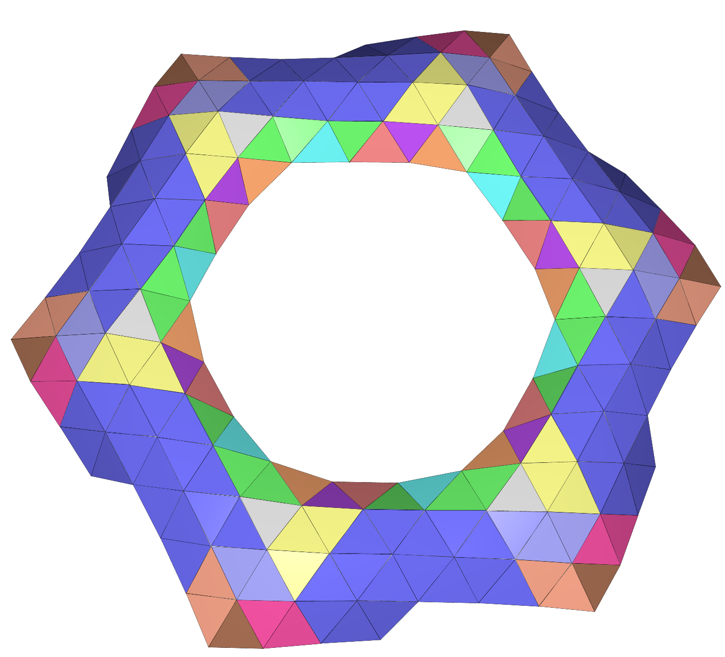
Re-meshed grid

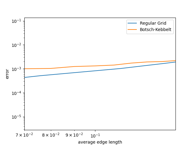
We also use the Botsch-Kebbelt re-meshing algorithm to re-mesh the regular grid, to generate more randomness in the alignment of the triangles to the principal curvature of the quadratic function. This algorithm takes in the surface as well as the desired average edge lengths of the the triangles in the mesh, and outputs to us a re-meshed surface. The images from left to right demonstrates what happens as we increase the average edge length that we pass in as a parameter.

Figure 16. Approximation of surface using a re-meshed grid with 0.07 desired edge length

Figure 17. Error plot of input desired re-meshed edge length and chamfer distance error

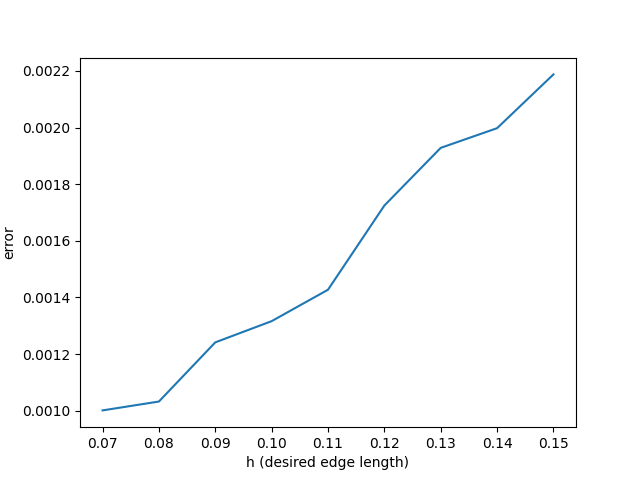
To make a more equal comparison, we converted the grid resolution to find the average edge length of the triangles in the regular grids and plotted its error together on a log-log graph. As we can see below, the regular grid does better than the Bosch-Kebbelt re-meshed grid. This is congruent with what we expected – that aligning the edges of the triangles would give us a lower error than just random orientations!

Figure 18. Comparison of the chamfer distance error for the regular grid and the botsch-kebbelt re-meshed grid

References:

[1] Bommes, David, et al. “Mixed-integer quadrangulation.” ACM Transactions on Graphics, vol. 28, no. 3, July 2009, pp. 1–10, doi:10.1145/1531326.1531383.

[2] Jakob, Wenzel, et al. “Instant Field-aligned Meshes.” ACM Transactions on Graphics, vol. 34, no. 6, Nov. 2015, pp. 1–15, doi:10.1145/2816795.2818078.

Author: Brittney Fahnestock and Yixin Lok
Project Mentor: Rulin Chen, Singapore University of Technology and Design
Volunteer Teaching Assistant: Kyle Onghai

Introduction

A K-set surface is a surface mesh that has each of its faces categorized into K discrete equivalence classes. Each discrete equivalence class corresponds to a fixed template polygon, and instances of these templates are used in place of the original mesh faces to form the final assembly structure. As we reduce the variety of building components, we improve the ease of fabrication and assembly – which is why we use K-set surfaces.

In this project, we use a hierarchical approach to cluster polygons and the ShapeOp library to optimize the given surfaces to produce K-set surfaces. Compared to previous works that aim to produce K-set surfaces in fixed topology (e.g., triangular surfaces or quadrilateral surfaces), our approach is able to create K-set surfaces with a variety of topologies.

Problem Formulation

Our input is a freeform surface and a chosen topology. Our output is a small set of discrete equivalence classes (i.e., template polygons) where the instances of template polygons can resemble the given surface as close as possible. Other design requirements include: 1) each polygon should be planar for easing fabrication and assembly process; 2) the intra-cluster variance should be converged to zero if possible.

Method

We use a cluster-and-optimize approach to produce K-set surfaces. In general, our approach includes four stages: (i) base mesh initialization; (ii) polygon clustering; (iii) mesh optimization; and (iv) template replacement.

(i) Base mesh initialization

In order to map the 2D pattern to the surface, we will utilize an as-rigid-as-possible algorithm. As-rigid-as-possible algorithm is utilized because of its ability to maintain the pattern while mapping.

Figure 1. Base mesh initialization.

(ii) Polygon clustering

We use a hierarchical approach to cluster polygons, i.e., we first cluster edges and diagonals, then we use the cluster labels of edges and diagonals to cluster polygons. The user may input two Ks to directly control the edges and diagonals, but may not directly control the K for polygons. Note that the premise for using this clustering approach is all the polygons should be planar. For each polygon cluster, we compute a centroid polygon template as the target polygon for the polygons in the cluster at the following optimization stage.

Figure 2. Our proposed hierarchical approach to clustering the base mesh polygons.

(iii) Mesh optimization

At this stage, our goal is to optimize base mesh to minimize the intra-cluster variances, i.e., each polygon should be as similar as its corresponding polygon template computed at the previous clustering stage. Our optimization function is as following:

\( E = E_{\text{polygon}} + E_{\text{surf}} + E_{\text{smth}} \)

where

\( E_{\text{polygon}} = E_{\text{edge}} + E_{\text{diagonal}} + E_{\text{planar}} \)

E_polygon: This term refers to the requirement that each polygon be optimized to closely match its corresponding centroid polygon template. Specifically, the length of each edge and diagonal should be as close as possible to the corresponding edge and diagonal in the centroid polygon, while maintaining the planar condition.

E_surf: This term refers to the requirement that the optimized surface should be as close as possible to the user-specified given surface.

E_smooth: This term refers to the requirement that the optimized surface should be as smooth as possible.

The geometry solver used is ShapeOp, as this library uses a state of the art physics solver that applies multiple constraints needed for shape optimization. In this project, ShapeOp helps us to convert the our proposed energy terms to the optimization functions represented by vertex positions.

(iv) Template replacement

After mesh optimization, we replace each polygon in the opimized surface with its corresponding template. In each polygon replacement process, we will find a best alignment orientation by calculating the minimal distance between vertices of polygons:

\( s(S_i, \tilde{S}_i) = \displaystyle\min_{k} \displaystyle\sum_{l=1}^{2L} \| \mathbf{v}_l – T_k(\tilde{\mathbf{v}}_l) \|^2 \)

After the polygon replacement, there will be errors since the conflicting optimization goals. Thanks to our proposed mesh optimization method, these errors are well minimized.

Figure 3. Errors after polygon replacement.

Result

We provide a series of K-set surfaces witn various surfaces and topologies. For each result, we provide the surfaces before and after centroid polygon replacement. The greater the similarity between the results before and after replacement, the more it demonstrates the effectiveness of our proposed method for producing K-set surfaces. We observe that there tends to be a trade off between a low K value and a low surface approximation error, as we replace each original mesh face with K templates.

References

[1] Fu, Chi-Wing, et al. “K-set tilable surfaces.” ACM transactions on graphics (TOG) 29.4 (2010): 1-6.

[2] Singh, Mayank, and Scott Schaefer. “Triangle surfaces with discrete equivalence classes.” ACM SIGGRAPH 2010 papers. 2010. 1-7.

[3] Chen, Rulin, et al. “Masonry shell structures with discrete equivalence classes.” ACM Transactions on Graphics 42.4 (2023).

[4] Deuss, Mario, et al. “ShapeOp—a robust and extensible geometric modelling paradigm.” Modelling Behaviour: Design Modelling Symposium 2015. Springer International Publishing, 2015.

K-set surface before replacement	K-set surface after replacement	Number of polygons	Number of unique polygons
		204	12
		423	20
		250	58
		289	51
		161	24