Categories
Math

Part I: Manifolds—Exploring Differential and Discrete Geometry Perspectives

ABSTRACT

In this three-part series, we rigorously explore the concept of manifolds through the perspectives of both differential geometry and discrete differential geometry. In Part I, we establish the formal definition of a manifold as a special type of topological space and present illustrative examples. In Part II, we introduce the additional structure needed to define differentiable manifolds. Finally, part III presents the discretization of manifolds within the framework of discrete differential geometry, where we approximate smooth manifolds using simplicial complexes or polygonal meshes. Looking at the concept from both perspectives is an opportunity to gain a deeper insight into both types of geometries. The series is nearly self-contained, requiring only a basic understanding of naive set theory and elementary calculus from the reader.

Introduction

A manifold is a special kind of topological space, so special, in fact, that mathematicians have given it its own name. The term “manifold” traces back to the Old English manigfeald and Proto-Germanic maniġfaldaz, meaning “many folds” or “layers.” This etymology descriptively captures the essence of what a manifold represents: a space with many dimensions or complexities, yet with a coherent structure. To define a manifold formally, we first introduce the concept of a general topological space. Only after this, we can talk about the specific properties that a topological space must have to be considered a manifold.

Topological Spaces

Definition. Let \( M \) be a set. Then a choice \( \mathcal{O} \subseteq \mathcal{P}(M) \) is called a topology on \( M \) if:

  1. \( \emptyset \in \mathcal{O} \) and \( M \in \mathcal{O} \);
  2. For \(\{U_i\}_{i=1}^n \subseteq \mathcal{O}\) \( \Rightarrow \bigcap \{U_i \}_{i=1}^n \in \mathcal{O}\)
  3. For any arbitrary collection of sets \( \mathcal{C} \subseteq \mathcal{O}\) \( \Rightarrow \bigcup \mathcal{C} \in \mathcal{O}\)

And the pair \( (M, \mathcal{O}) \) is called a topological space.

Abuse of Notation. In this note, sometimes we abbreviate \(M, \mathcal{O}\) by just \(M\), leaving the topology \( \mathcal{O}\)
implicit.

In mathematics, a topology on a set provides the weakest structure needed to define the two very important notions of convergence of sequences to points in a set, and of continuity of maps between two sets. Unless \( |M|=1 \). There are many different topologies one could establish on a set on the same set. Depending on what topology you have on \(M\), the notion of continuity and convergence changes accordingly.

The following table shows us how many different topologies one can establish on a set based on its cardinality.

\( |M| \)Number of Topologies
11
24
329
4355
56,942
6209,527
79,535,241

Examples of Topologies

  1. Chaotic (trivial) topology: For the set \( M = \{a, b, c\} \), the chaotic topology includes only the entire set and the empty set: \( \mathcal{O} = \{\emptyset, M\} \). This topology is called “chaotic” because it has the least structure, and can be defined on any set.
  2. Discrete Topology: For the set \( M = \{a, b, c\} \), the discrete topology includes every possible subset of \( M \): \( \mathcal{O} = \{\emptyset, \{a\}, \{b\}, \{c\}, \{a, b\}, \{a, c\},\{b, c\}, \{a, b, c\}\}\). This topology provides the most structure, and can be defined on any set.
  3. Standard Topology on \( \mathbb{R} \) (Open Interval Topology): For the set \( M = \mathbb{R} \) (the real numbers), the standard topology is generated by open intervals \( (a, b) \) where \( a, b \in \mathbb{R} \) and \( a < b \): \( \mathcal{O} = \{U \subseteq \mathbb{R} \mid U \text{ is a union of open intervals } (a, b)\}\)

Just as sets are distinguished from each other based on one important property—the cardinality of sets—in set theory, we can define properties that help distinguish one topological space from another. There are many such topological properties for this purpose. We will present those needed to distinguish a topological space that is a manifold from one that is not, namely, the separation, compactness, and paracompactness properties.

Separation, Compactness, and Paracompactness of Topological Spaces

Separation Properties:

Separation properties are used to distinguish points and sets within a topological space, providing a way to understand how “separate” or “distinct” different points or subsets are. To illustrate, consider
\(M = \{a, b, c\}\) and the topology \( \mathcal{O} = \{\phi, \{a, b, c\}\}\). This topology is fairly “blind to its element”: it can not tell apart any of the points \(a, b, c\)! But any metric space can tell its points apart
(because \(d(x, y) > 0 \) when \( x \neq y\)). While we focus on one specific type of separation property—the \(T_2\) Hausdorff property—there are many other separation properties (many \(Ts\)), some stronger while others are weaker than \(T_2\), that also play important roles in topology.

Definition: A topological space \( (M, \mathcal{O}) \) is called a Hausdorff space (or \(T_2\) space) if for any two distinct points \( p, q \in O \), there exist disjoint open neighborhoods \( U \) and \( V \) such that \( p \in U \) and \( q \in V \). That is, the space satisfies the following condition:

For any \( p, q \in \mathcal{O}\) with \(p \neq q,\) there exist disjoint open sets \(U\) and \(V\) such that \(p \in U\) and \(q \in V. \)

Example: Consider the topological space \( (\mathbb{R}^2, \mathcal{O}) \), where \( \mathcal{O} \) is the standard topology on \( \mathbb{R}^2 \). This space is \(T_2\) Hausdorff. The standard topology \( \mathcal{O} \) on \( \mathbb{R}^2 \) is the collection of all unions of open balls.

An open ball centered at a point \( (x_0, y_0) \) with radius \( r > 0 \) is:
\( B((x_0, y_0), r) = \{ (x, y) \in \mathbb{R}^2 \mid \sqrt{(x – x_0)^2 + (y – y_0)^2} < r \} \)

And indeed, \( \mathbb{R}^2 \) has the\(T_2\) (Hausdorff) property since given any two distinct points in \( \mathbb{R}^2 \), you can always find two open balls that do not overlap.

More generally, the topological space \( (\mathbb{R}^d, \mathcal{O} )\) is \(T_2\) Hausdorff where \( \mathcal{O} \) is its standard topology.

Compactness, and Paracompactness:

Definition. Let \( (M, \mathcal{O}) \) be a topological space. An open cover of \( M \) is an arbitrary collection of open sets \( \{ U_{\alpha \in A} \}\) from \( \mathcal{O}\) (possibly infinite or finite) such that: \[ M = \bigcup_{\alpha \in A} U_{\alpha} \]

A subcover is exactly what it sounds like: it takes only some of the \(U_{\alpha \in A}\), while ensuring that \(M\) remains covered.

Definition. A topological space ( \(M, \mathcal{O}\) ) is called compact if every open cover of \( M \) has a finite subcover (i.e. there exists \( F \subset A \) such that: \(M = \bigcup_{\alpha \in F} U_{\alpha}\) where \(F\) is finite).

Compactness is a property that generalizes the notion of closed and bounded sets in Euclidean space. A topological space is compact if every open cover of the space has a finite subcover. This means that, no matter how the space is covered by open sets, it is possible to select a finite number of those sets that still cover the entire space. Compact spaces have several important properties.

In many mathematical contexts, when developing and proving new theorems within the framework of topological spaces, it is common to first address the case where the space is compact. Once the theorem/proof is established for compact spaces, efforts are then made to extend the result to non-compact spaces. Sometimes it is not possible to do the extension. On the other hand, paracompactness is a generalization of compactness (i.e, a much weaker notion) and rarely is it the case to find a topological space that is not paracompact.

Paracompactness:

Definition. A topological space \( (M, \mathcal{O}) \) is called paracompact if every open cover has an open refinement that is locally finite.

Given an open cover \( \{ U_{\alpha \in A} \}\) of \(M\), an open refinement \( { V_{\beta} }_{\beta \in B} \) of this cover is another open cover where every \( V_{\beta} \) is contained in some \( U_{\alpha} \) (i.e. \(\{ V_{\beta} \}_{\beta \in B}\) is a refinement if \( V_{\beta} \subset U_{\alpha} \text{ for some } \alpha \in A.\))

In other words, \( { V_{\beta} }_{\beta \in B} \) is a finer cover than \( \{ U_{\alpha \in A} \}\), meaning that each open set in the refinement is more “localized” or “smaller” in some sense compared to the original cover.

Definition. The refinement is said to be locally finite if every point in \( M \) has a neighborhood that intersects only finitely many of the sets \( V_{\beta} \).

This means that around any given point, only a finite number of the open sets in the cover are “active” or have non-empty intersections with the neighborhood.

In summary: Compactness ensures that any cover can be reduced to a finite cover, while paracompactness ensures that any cover can be refined to a locally finite cover. Compactness deals with the ability to reduce the size of a cover, while paracompactness deals with the ability to organize the cover more effectively without too much local overlap.

Now, we are ready to lay down the formal definition of a manifold!

Manifolds

Definition: A paracompact, Hausdorff topological space ( \(M, \mathcal{O}\) ) is called a (d)-dimensional manifold if for every point \( p \in M \), there exists a neighborhood \( U(p) \) of \( p \) and a homeomorphism \( \varphi: U(p) \to \varphi(U(p) ) \subset \mathbb{R}^d \). In this case, we also write dim \(M\)= \( d \).

What are homeomorphisms? Homeomorphism (Homeos) are structure-preserving maps between topological spaces. Formally, we say that a map \( \varphi: (M, \mathcal{O}_M) \to (N, \mathcal{O}_N) \) is called a homeomorphism if it satisfies the following conditions:

  • \( \varphi: (M, \mathcal{O}_M) \to (N, \mathcal{O}_N) \) is a bijection
  • \( \varphi: (M, \mathcal{O}_M) \to (N, \mathcal{O}_N) \) is continuous
  • The inverse map \( \varphi^{-1}: (N, \mathcal{O}_N) \to (M, \mathcal{O}_M) \) is also continuous.

This definition tells us that a d-manifold is a special type of a topological space where we can distinguish between its subspaces, and it gives us two equivalent ways to think about it:

  • Locally: for any arbitrary point \(p \in M\), you can always find an open set that contains it and this open set can be mapped by some homeo to a subset of \(\mathbb{R}^d\). For example, to someone standing on the surface of the Earth, the Earth looks much like \(\mathbb{R}^2\).
  • Globally: there exists an open cover \( \{ U_{\alpha \in A} \}\) (possibly infinite) of \(M\) such that every \(U_{\alpha}\) is mapped by some homeo to a subset of \(\mathbb{R}^d\). For example, from outer space, the Earth can be covered by two hemispherical pancakes.

Examples of Manifolds

  1. The sphere \(S^2\) is a 2-manifold: every point in the sphere has a small open neighborhood that looks like a subset of \(\mathbb{R}^2\). One can cover the Earth with just two hemispheres, and each hemisphere is homeomorphic to a disk in \(\mathbb{R}^2\).
  2. The circle \(S^1\) is a 1-manifold; every point has an open neighborhood that looks like an open interval.
  3. The torus \(T^2\), and Klein bottle are 2-manifold too.

A non-example of a topological space that is not a manifold is the \(n\)-dimensional disk \(D^n\), because it has a boundary; points on the boundary do not have open neighborhoods that can be mapped by some homeo to a subset of \(\mathbb{R}^n\).

Definition. The closed n-dimensional disk, denoted by \( D^n \), is defined as the set of all points \( \mathbf{x} \in \mathbb{R}^n \) such that the Euclidean norm of \( \mathbf{x} \) is less than or equal to 1. Formally,
\[ D^n = \{ \mathbf{x} \in \mathbb{R}^n \mid |\mathbf{x}| \leq 1 \} \]
where \( |\mathbf{x}| = \sqrt{x_1^2 + x_2^2 + \dots + x_n^2} \) is the Euclidean norm of the vector \( \mathbf{x} = (x_1, x_2, \dots, x_n) \).

Additional terminology: Atlases and Charts

The Terminology of a Chart on a \(d\)manifold:

Let \(M\) be a \(d\)-manifold then, a chart on \(M\) is a pair \( (U, \varphi) \), where:

  • \( U \) is an open subset of \( M \).
  • \( \varphi: U \to \varphi(U) \subset \mathbb{R}^d \) (often called the coordinate map or coordinate chart) is a homeomorphism.

The component functions of \( \varphi: U \to \varphi(U) \subset \mathbb{R}^d \) are the mappings:

\[\varphi^{i}: U \to \mathbb{R}\]
\[p \mapsto proj_i(\varphi(p))\]

For \(1 \leq i \leq d\), where \(proj_i(\varphi(p))\) is the \(i\)-th component of \( \varphi (p) \in \mathbb{R}^d\).

This means that the map \( \varphi \) takes every point \(p\) in \( U \) and assigns it coordinates \(proj_i(\varphi(p))\) in \( \mathbb{R}^d = \mathbb{R}\times \mathbb{R} \times \dots \times \mathbb{R}\) ) ( \(d\) times) with respect to the chart \((U, \varphi) \).

Remarks.

  1. Notice that the paragraph above does not introduce any new information beyond what is contained in the definition of a \(d\)-topological manifold. This is why a “chart” is more of a terminology than a definition—though it is a useful one.
  2. We can see by now that there can exist a set \( \mathscr{A}\) of charts for each open set in the open cover \( \{ U_{\alpha \in A} \}\) of \(M\), and there will be many charts that overlap because Different charts may be needed to cover the entire manifold because a single chart might not be able to cover the entire surface of a sphere without singularities or overlaps.

Definition. An atlas of a manifold \( M \) is a collection \( \mathscr{A} := \{(U_\alpha, \varphi_\alpha) \mid \alpha \in A\} \) of charts such that:\[\bigcup_{\alpha \in A} U_\alpha = M.\]

Well, where do you think the words “chart” and “atlas” come from? 🙂

So what happens then if charts overlap? A natural map called the transition map displays itself naturally and is always continuous as a result of the original definition of the topological \(d\)-manifold.

Definition. Two charts \((U_1, \varphi_1)\) and \((U_2, \varphi_2)\) are called \(C^0\)-compatible if either:

  1. \(U_1 \bigcap U_2 \neq \phi \)
  2. \(U_1 \bigcap U_2 = \phi \): the (transition) map \( \varphi_2 \circ \varphi_1^{-1} : \varphi_1(U_1 \bigcap U_2) \to \varphi_2(U_1 \bigcap U_2)\) is continuous

By definition, one can go from \(U_1\) into \(\varphi_1 (U_1) \subseteq \mathbb{R}^d\), and similarly one can go from \(U_2\) into \(\varphi_2 (U_2) \subseteq \mathbb{R}^d\). For all the points in the \( U_1 \cap U_2 \), one could use either apply \(\varphi_1\) or \( \varphi_2 \) to land in the subsets \( \varphi_1 (U_1 \cap U_2) \) or \( \varphi_2 (U_1 \cap U_2) \) of \( \mathbb{R}^d \). All of a sudden, we constructed a map that goes from \( \varphi_2 \circ \varphi_1^{-1}: \mathbb{R}^d \to \mathbb{R}^d\) and this map is always continuous

This definition seems redundant and this is true, it applies to every pair of charts. However, it is just a “warm up” since we will later refine this definition and define the differentiability of maps on a manifold in terms of \(C^k\)-compatibility of charts.

Example. Consider a 2-dimensional manifold ( M ), such as the surface of a globe (a sphere). One chart ( (U_1, \varphi_1) ) might cover the Northern Hemisphere, with ( \varphi_1 ) assigning each point in ( U_1 ) latitude and longitude coordinates. Another chart ( (U_2, \varphi_2) ) might cover the Southern Hemisphere. In the overlap ( U_1 \cap U_2 ), the transition map ( \varphi_2 \circ \varphi_1^{-1} ) converts coordinates from the Northern Hemisphere chart to the Southern Hemisphere chart.

Remark. The structure of a topological \(d\)-manifold \(M\) allows us to distinguish subspaces (sub-manifolds) from each other and provides the framework to discuss the continuity of functions defined on \(M\). For example, if you have a curve \( c: \mathbb{R} \to M\) on the manifold, a function \( \mu: \mathbb{R} \to M \) or even a map \(\phi: M \to M\) you can talk about the continuity of \(c\), \(\mu\) and \(\phi\). However, the topological structure alone is not sufficient to discuss their differentiability. To do so, we need to impose an additional structure on \(M\), such as a smooth structure, to define and talk about differentiability.

In part II, we will talk more about Differentiable Manifolds.

Bibliography:

Frederic Schuller (Director). (2015, September 22). Topological manifolds and manifold bundles- Lec 06—Frederic Schuller [Video recording]. https://www.youtube.com/watch?v=uGEV0Wk0eIk

Ananthakrishna, G., Conway, A., Ergen, E., Floris, R., Galvin, D., Hobohm, C., Kirby, R., Kister, J., Kosanović, D., Kremer, C., Lippert, F., Merz, A., Mezher, F., Niu, W., Nonino, I., Powell, M., Ray, A., Ruppik, B. M., & Santoro, D. (n.d.). Topological Manifolds.

Munkres, J. R. (2000). Topology (2nd ed.). Pearson.

Categories
Uncategorized

The Origins of ‘Bug’ and ‘Debugging’ in Computing and Engineering

By Ehsan Shams

During these six fascinating weeks at SGI, I have said and heard the words “bug” and “debugging” so often that if I had an inch for every time, I could go from Egypt to Tahiti and back a few dozen times. Haha! As an etymology enthusiast, I couldn’t resist digging into the origins of these terms. Here’s what I discovered.

The use of the term “bug” in engineering and technology contexts dates back to at least the 19th century. The term was used by Thomas Edison in a letter written in 1878 to Tivadar Puskás here, in which Edison referred to minor engineering flaws or difficulties as “bugs,” implying that these small issues were natural in the process of invention and experimentation.

Specifically, Edison wrote about the challenges of refining his inventions in this letter, stating:

“It has been just so in all of my inventions. The first step is an intuition—and comes with a burst, then difficulties arise—this thing gives out and [it is] then that ‘bugs’—as such little faults and difficulties are called—show themselves, and months of intense watching, study and labor are requisite before commercial success—or failure—is certainly reached.”

Thomas Edison and His ‘Insomnia Squad’: Debugging Inventions All Night and Napping Through the Day. Photo: Bettmann/Getty Images

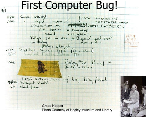
The term gained further prominence in the mid-20th century, especially in computing when engineers working on the Mark II computer at Harvard University in 1947, and found that the computer was malfunctioning. Upon investigation, Grace Hopper discovered that a moth had become trapped in one of the machine’s relays (Relay #70 on Panel “F” of the Harvard Mark II Aiken Relay Calculator), causing a problem, and took a photo of it and documented it.

Harvard Mark II Aiken Relay Calculator

The engineers removed the moth and taped it into the log book with the note: “First actual case of a bug being found.” While the term “bug” had already been in use to describe technical issues or glitches, this incident provided a literal example of the term, and it is often credited with popularizing the concept of “de-bugging” in computer science.

The logbook, complete with the taped moth, is preserved in the Smithsonian National Museum of American History as a notable piece of computing history. This incident symbolically linked the term “bug” with computer errors in popular culture and the history of technology.

Turns out that the term “bug” has a rich etymology, originating in Middle English where it referred to a ghost or hobgoblin that troubled and scared people. By the 16th century, “bug” started to be used to describe insects, particularly those that were seen as pests, such as bedbugs which cause discomfort, then in the 19th century, engineers adopted “bug” as a metaphor for small flaws or defects in machinery, likening these issues to tiny pests that could disrupt a system’s operation and cause discomfot.

It’s hilarious how the word “bug” still sends shivers down our spines—back then, it was ghosts and goblins, and now it could be a missing bracket hiding somewhere in a hundred-something-line program, a variable you forgot to declare, or an infinite loop that makes your code run forever!

References:

  1. Edison, T. (1878). Letter to Tivadar Puskás. The Thomas Edison Papers. Rutgers University. https://edisondigital.rutgers.edu/document/D7821ZAO#?xywh=-2%2C-183%2C940%2C1090
  2. National Geographic Education. (n.d.). World’s first computer bug. Retrieved August 18, 2024, from https://education.nationalgeographic.org/resource/worlds-first-computer-bug
  3. Hopper, G. M. (1987). The Mark II computer and the first ‘bug’. Proceedings of the ACM History of Programming Languages Conference.


Categories
Math

The Area of a Circle

Author: Ehsan Shams (Alexandria University, Egypt)

“Since people have tried to prove obvious propositions,
they have discovered that many of them are false.”
Bertrand Russell

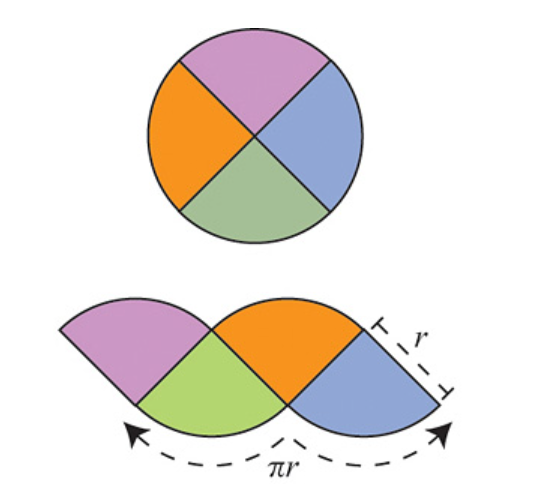
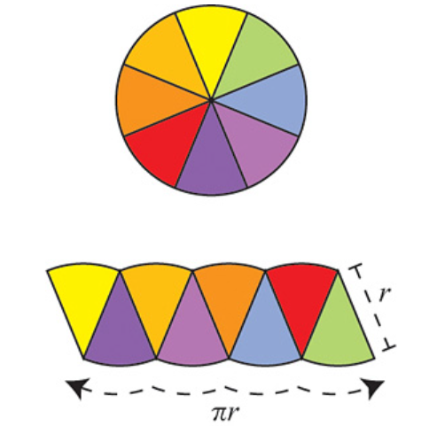
Archimedes proposed an elegant argument indicating that the area of a circle (disk) of radius \(r\) is \( \pi r^2 \). This argument has gained attention recently and is often presented as a “proof” of the formula. But is it truly a proof?

The argument is as follows: Divide the circle into \(2^n\) congruent wedges, and re-arrange them into a strip, for any \( n\) the total sum of the wedges (the area of the strip) is equal to the area of the circle. The top and bottom have arc length \( \pi r \). In the limit the strip becomes a rectangle, meaning as \( n \to \infty \), the wavy strip becomes a rectangle. This rectangle has area \( \pi r^2 \), so the area of the circle is also \( \pi r^2 \).

These images are taken from [1].

To consider this argument a proof, several things need to be shown:

  1. The circle can be evenly divided into such wedges.
  2. The number \( \pi \) is well-defined.
  3. The notion of “area” of this specific subset of \( \mathbb{R}^2 \) -the circle – is well-defined, and it has this “subdivision” property used in the argument. This is not trivial at all; a whole field of mathematics called “Measure Theory” was founded in the early twentieth century to provide a formal framework for defining and understanding the concept of areas/volumes, their conditions for existence, their properties, and their generalizations in abstract spaces.
  4. The limiting operations must be made precise.
  5. The notion of area and arc length is preserved under the limiting operations of 4.

Archimedes’ elegant argument can be rigorised but, it will take some of work and a very long sheet of paper to do so.

Just to provide some insight into the difficulty of making satisfactory precise sense of seemingly obvious and simple-to-grasp geometric notions and intuitive operations which are sometimes taken for granted, let us briefly inspect each element from the above.

Defining \( \pi \):

In school, we were taught that the definition of \( \pi \) is the ratio of the circumference of a circle to its diameter. For this definition to be valid, it must be shown that the ratio is always the same for all circles, which is
not immediately obvious; in fact, this does not hold in Non-Euclidean geometry.

A tighter definition goes like this: the number \( \pi \) is the circumference of a circle of diameter 1. Yet, this still leaves some ambiguity because terms like “circumference,” “diameter,” and “circle” need clear definitions, so here is a more precise version: the number \( \pi \) is half the circumference of the circle \( \{ (x,y) | x^2 + y^2 =1 \} \subseteq \mathbb{R}^2 \). This definition is clearer, but it still assumes we understand what “circumference” means.

From calculus, we know that the circumference of a circle can be defined as a special case of arc length. Arc length itself is defined as the supremum of a set of sums, and in nice cases, it can be exactly computed using definite integrals. Despite this, it is not immediately clear that a circle has a finite circumference.

Another limiting ancient argument that is used to estimate and define the circumference of a circle and hence calculating terms of \( \pi \) to some desired accuracy since Archimedes was by using inscribed and circumscribed regular polygons. But still, making a precise sense of the circumference of a circle, and hence the number \( \pi \), is a quite subtle matter.

The Limiting Operation:

In Archimedes’ argument, the limiting operation can be formalized by regarding the bottom of the wavy strip (curve) as the graph of a function \(f_n \), and the limiting curve as the graph of a constant function \(f\). Then \( f_n \to f \) uniformly.

The Notion of Area:

The whole of Euclidean Geometry deals with the notions of “areas” and “volumes” for arbitrary objects in \( \mathbb{R}^2 \) and \( \mathbb{R}^3 \) as if they are inherently defined for such objects and merely need to be calculated. The calculation was done by simply cutting the object into finite simple parts and then rearranging them by performing some rigid motion like rotation or translation and then reassembling those parts to form a simpler body which we already know how to compute. This type of Geometry relies on three hidden assumptions:

  • Every object has a well-defined area or volume.
  • The area or volume of the whole is equal to the sum of the areas or volumes of its parts.
  • The area or volume is preserved under such re-arrangments.

This is not automatically true for arbitrary objects; for example consider the Banach-Tarski Paradox. Therefore, proving the existence of a well-defined notion of area for the specific subset describing the circle, and that it is preserved under the subdivision, rearrangement, and the limiting operation considered, is crucial for validating Archimedes’ argument as a full proof of the area formula. Measure Theory addresses these issues by providing a rigorous framework for defining and understanding areas and volumes. Thus, showing 1,3, 4, and the preservation of the area under the limiting operation requires some effort but is achievable through Measure Theory.

Arc Length under Uniform Limits:

The other part of number 5 is slightly tricky because the arc length is not generally preserved under uniform limits. To illustrate this, consider the staircase curve approximation of the diagonal of a unit square in \( \mathbb{R}^2 \). Even though as the step curves of the staircase get finer and they converge uniformly to the diagonal, their total arc length converges to 2, not to \( \sqrt{2} \). This example demonstrates that arc length, as a function, is not continuous with respect to uniform convergence. However, arc length is preserved under uniform limits if the derivatives of the functions converge uniformly as well. In such cases, uniform convergence of derivatives ensures that the arc length is also preserved in the limit. Is this provable in Archimedes argument? yes with some work.

Moral of the Story:

There is no “obvious” in mathematics. It is important to prove mathematical statements using strict logical arguments from agreed-upon axioms without hidden assumptions, no matter how “intuitively obvious” they seem to us.

“The kind of knowledge which is supported only by
observations and is not yet proved must be carefully
distinguished from the truth; it is gained by induction, as
we usually say. Yet we have seen cases in which mere
induction led to error. Therefore, we should take great
care not to accept as true such properties of the numbers
which we have discovered by observation and which are
supported by induction alone. Indeed, we should use such
a discovery as an opportunity to investigate more exactly
the properties discovered and to prove or disprove them;
in both cases we may learn something useful.”
L. Euler

“Being a mathematician means that you don’t take ‘obvious’
things for granted but try to reason. Very often you will be
surprised that the most obvious answer is actually wrong.”
–Evgeny Evgenievich

Bibliography

  1. Strogatz, S. (1270414824). Take It to the Limit. Opinionator. https://archive.nytimes.com/opinionator.blogs.nytimes.com/2010/04/04/take-it-to-the-limit/
  2. Tao, T. (2011). An introduction to measure theory. Graduate Studies in Mathematics. https://doi.org/10.1090/gsm/126
  3. Pogorelov, A. (1987). Geometry. MIR Publishers.
  4. Blackadar, B. (2020). Real Analysis Notes
Categories
Math Research

Spline Construction with Closed-form Arc-Length Solution: A Guided Tour

Author: Ehsan Shams (Alexandria Univerity, Egypt)
Project Mentor: Sofia Di Toro Wyetzner (Stanford University, USA)
Volunteer Teaching Assistant: Shanthika Naik (CVIT, IIIT Hyderabad, India)

In my first SGI research week, I went on a fascinating exploratory journey into the world of splines under the guidance of Sofia Wyetzner, and gained an insight into how challenging yet intriguing their construction can be especially under tight constriants such as the requirement for a closed-form expression for their arc-length. This specific construction was the central focus of our inquiry, and the main drive for our exploration.

Splines are important mathematical tools for they are used in various branches of mathematics, including approximation theory, numerical analysis, and statistics, and they find applications in several areas such as Geometry Processing (GP). Loosely speaking, such objects can be understood as mappings that take a set of discrete data points and produce a smooth curve that either interpolates or approximates these points. Thus, it becomes natural immediately to see that they are of great importance in GP since, in the most general sense, GP is a field that is mainly concerned with transforming geometric data1 from one form to another. For example, splines like Bézier and B-spline curves are foundational tools for curve representation in computer graphics and geometric design (Yu, 2024).

Having access to arc lengths for splines in GP is essential for many tasks, including path planning, robot modeling, and animation, where accurate and realistic modeling of curve lengths is critically important. For application-driven purposes, having a closed formula for arc-length computation is highly desirable. However, constructing splines with this arc-length property that can interpolate \( k \) arbitrary data points reasonably well is indeed a challenging task.

Our mentor Sofia, and Shanthika guided us through an exploration of a central question in spline formulation research, as well as several related tangential questions:

Our central question was:

Given \( k \) points, can we construct a spline that interpolates these points and outputs the intermediate arc-lengths of the generated, curve, with some continuity at control points?

And the tangential ones were:

1. Can we achieve \( G^1 \) / \( C^1\) / \( G^2 \) / \(C^2\) continuity at these points with our spline?
2. Given \(k\) points and a total arc-length, can we interpolate these points with the given arc-length in \( \mathbb{R}^2 \)?

In this article, I will share some of the insights I gained from my first week-long research journey, along with potential future directions I would like to pursue.

Understanding Splines and their Arc-length

What are Splines?

A spline is a mapping \( S: [a,b] \subset \mathbb{R} \to \mathbb{R}^n \) defined as:

\( S(t) = \begin{cases} s_1(t) & \text{for } t \in [t_0, t_1] \\ s_2(t) & \text{for } t \in [t_1, t_2] \\ \vdots \\ s_n(t) & \text{for } t \in [t_{n-1}, t_n] \end{cases} \)

where \( a = t_0 < t_1 < \cdots < t_n = b \), and \( s_i: [t_i, t_{i+1}] \to \mathbb{R}^n \) are defined such that, \(S(t)\) ensures \( C^k \) continuity at each internal point \( t_j \), meaning:

\( s_{i-1}^{(m)}(t_j) = s_i^{(m)}(t_j) \) for \( m = 0,1 \dots, k \)

where \( s_{i-1}^{(m)} \) and \( s_i^{(m)} \) are the \( m \)-th derivatives of \( s_{i-1}(t) \) and \( s_i(t) \) respectively.

In other words, a spline is a mathematical construct used to create a smooth curve \( S(t) \) by connecting a sequence of simpler piecewise segments \( s_i(t) \) in a continuous manner. These segments \( s_i(t) \) for \( i = 1, 2, \ldots, n \) are defined on subintervals \( [t_i, t_{i+1}] \) of the parameter domain, and are carefully joined end-to-end. The transitions at the junctions \( \{ t_i \}_{i=1}^{n-1} \) (also known as control points) maintain a desired level of smoothness, typically defined by the continuity of derivatives up to order \( k \) on \( \{s_i(t)\}_{i=1}^n \).

One way to categorize splines is based on the types of functions \(s_i\) they incorporate. For instance, some splines utilize polynomial functions such as Bézier splines and B-splines, while others may employ trigonometric functions such as Fourier splines or hyperbolic functions. However, the most commonly used splines in practice are those based on polynomial functions, which define one or more segments. Polynomial splines are particularly valuable in various applications because of their computational simplicity and flexibility in modeling curves.

Arc Length Calculation

Intuitively, the notion of arc-length of a curve2 can be understood as the numerical measurement of the total distance traveled along the curve from one endpoint to another. This concept is fundamental in both calculus and geometry because it provides a way to quantify the length of some curves, which may not be a straight line. To calculate the arc length of smooth curves, we use integral calculus. Specifically, we apply a definite integral formula – (presented in the following theorem) but, let us first define the concept formally.

Definition. Let \( \gamma : [a, b] \to \mathbb{R}^n \) be a parametrized curve, and \( P = \{ a = t_0, t_1, \dots, t_n = b \} \) a partition of \( [a, b] \). The polygonal approximate3 length of \( \gamma \) from \(P\) is given by the sum of the Euclidean distances between the points \( \gamma(t_i)\) for \( i = 0, 1, \dots, n \):

\(L_P(\gamma) = \sum_{i=0}^{n} |\gamma(t_{i+1}) – \gamma(t_i)|\)

where \( | \cdot | \) denotes the Euclidean norm in \( \mathbb{R}^n \). This polygonal approximation becomes a better estimate of the actual length of the curve as the partition \( P\) becomes finer (i.e., as the maximum distance between successive \( t_i \) tends to zero). The actual length of the curve can be defined as:

\( L(\gamma) = \sup_P L_P(\gamma) \)

If the curve \( \gamma \) is sufficiently smooth, the actual length of the curve can be computed using definite integration as shown in the following theorem.

Arc Length Theorem. Let \( \gamma : [a, b] \to \mathbb{R}^n \) be a \( C^1 \) curve. The arc length \( L(\gamma) \) of \(\gamma\) is given by:

\( L(\gamma) = \int_a^b |\gamma'(t)| \, dt \)

where \(\gamma'(t) \) is the derivative of \(\gamma\) with respect to \(t\).

The challenge

As mentioned earlier, in the context of spline construction for GP tasks, ideally one is interested in constructing splines that have closed-form solutions for their arc length (a formula for computing their arc-length). However, curves with this property for their arc-length are relatively rare because the arc length integral often leads to elliptic integrals4 or other forms that do not have elementary antiderivatives. However, there are some curves for which the arc length can be computed exactly using a closed formula. Here are some examples: Straight lines, circles, and parabolas under certain conditions have closed-form solutions for arc length.

Steps to tackle the central question …

Circular Splines: A Starting Point.

In day one, our mentor Sofia went with us through a paper titled “A Class of \(C^2 \) Interpolating Splines” (Yuksel, 2020). In this work, the author introduces a novel class of non-polynomial parametric splines to interpolate given \( k \) control points. Two components define their class construction: interpolating functions and blending functions (defined later). Each interpolating function \(F_j \in \{F_i \}_{i=1}^n\) defines three consecutive control points, and the blending functions \( \{ B_i \}_{i=1}^m \) combines each two consecutive interpolating functions, forming a smooth curve between two control points. The blending functions are chosen so that \( C^2 \)-continuity everywhere is ensured independent of the choice of the interpolating functions. They use trignometric blending functions.

This type of formulation was constructed to attain some highly desirable properties in the resulting interpolating spline not previously demonstrated by other spline classes, including \( C^2 \) continuity everywhere, local support, and the ability to guarantee self-intersection-free curve segments regardless of the placement of control points and form perfect circular arcs. This paper served as a good starting point in light of the central question under consideration because among the interpolating functions they introduce in their paper are circular curves which have closed formulas for arc-length computation. In addition, it gives insight into the spline formulation practice. However, circular interpolating functions are not without their limitations; their constant curvature makes them difficult to reasonably interpolate arbitrary data, and they look bizarre sometimes.

Interesting note: The earliest documented reference – to the best of my knowledge – discussing the connection of two interpolating curves with a smooth curve dates back to Macqueen’s research in 1936 (MacQueen, 1936) Macqueen’s paper, titled “On the Principal Join of Two Curves on a Surface,” explores the concept of linking two curves on a surface.

Here is a demo constructed by the author to visualize the resulting output spline from their class with different interpolating functions, and below is me playing with the different interpolating functions, and looking at how bizarre the circular interpolating function looks when you throw out data points in an amorphus way.

While playing with the demo, the Gnomus musical track by Modest Mussorgsky was playing in parallel in the back of my mind so I put there for you too. It is a hilarious coincidence that the orchestra goes mad when it is the circular spline’s turn to interpolate the control points, and it does so oddly and bizarrely than the other splines in question. It even goes beyond the boundary of the demo. Did you notice that? 🙂

By the end of the day, I was left with two key inquiries, and a starting point for investigating them:

How do we blend desirable interpolating functions to construct splines with the properties we want? Can we use a combination of circular and elliptical curves to achieve more flexible and accurate interpolation for a wider variety of data points while maintaining a closed form for their arc length? What other combinations could serve us well?
I thought to myself: I should re-visit my functional analysis course as a starting point to think about this in a clear way.

From day two to five, we followed a structured yet not restrictive approach, akin to “we are all going to a definite destination but at the same time, everyone could stop by to explore something that captured their attention along the way if they want to and share what intrigued them with others”. This approach was quite effective and engaging:

  • Implementing a User-Interactive: Our first task was to develop a simple user interface for visualizing existing spline formulations. My SGI project team and friends—Charuka Bandara, Brittney Fahnestock, Sachin Kishan, and I—worked on this in Python (for Catmull-Rom splines) and MATLAB (for Cubic and Quadratic splines). This tool allowed us to visualize how different splines behave and change shape whenever the control points change, also restored my love for coding as I have not coded in a while … you know nothing is more joyful than watching your code executing exactly what you want it to do, right?
    Below is a UI for visualizing a Cubic Spline. Find the UI for the Quadratic Spline, and the Catmull-Rom here.
Interactive Cubic Spline
  • Exploring Blending Functions Method: As a natural progression towards our central inquiry, and a complementary task to reading Yuksel’s paper, we eventually found our way to exploring blending functions—a topic I had been eagerly anticipating.

Here, I decided to pause and explore more about the blending function method in spline formulation.

The blending function method, is a method that provides a way to construct a spline \( S(t) \) as a linear combination of a set of control points \( \{p_i(t)\}_{i=1}^n \) and basis functions (blending functions) \( \{B_i(t)\}_{i=1}^n \) in the following manner:

\( S(t) = \sum_{i=1}^n p_i B_i(t)\) (*)

where:
\( t \): is the parameter defined over the interval of interest \( [a,b] \)

These blending functions \(B_i(t)\) typically exhibit certain properties that govern, for example, the smoothness, continuity, shape, and preservation of key characteristics that we desire in the resulting interpolating splines. Thus, by carefully selecting and designing those blending functions, it is possible to tailor the behaviour of spline interpolation to meet the specific requirements and achieve desired outcomes.

Below are some of the properties of important blending functions:

  1. Partition of Unity: \( \sum_{i=1}^n B_i(t) =1, \forall t \in [a,b] \), also called coordinate system independent. This property is important because it provides a convex combination of the control points in question, and this is something you need to ensure that the curve does not change if the coordinate changes, one way to visualize this is by imagining that the control points in questions are beads sitting in an amorphous manner on a sheet of paper and the interpolating curve as a thread going through them, and you move the sheet of paper around, what we need is that the thread that goes through these beads does not move around as well, and this is what this property means. Notice that if you pick an arbitrary set of blending functions, this property is not immediately actualized, and the curve would change.
  2. Local Support: Each blending function \( B_i(t) \neq 0 \forall t \in I and i=1,2, … , n \) where \(I \subset [a,b] \) is the interval of interest and vanishes everywhere else on the domain. This property is important because it ensures computational efficiency. With this property actualized in one’s blending functions, one does not have to worry about consequences on their interpolating curve if they are to modify one control point .. for it will only affect a local region in the curve, and not the entire curve.
  3. Non-negativity: Blending functions are often non-negative over the domain of definition \( [a,b] \). This property is called convex hull. It is important for maintaining stability and predictability of the interpolating spline. It prevents the curve from oscillating wildly or provides unfaithful representation of the data point in question.
  4. Smoothness: Blending functions dictate the overall smoothness of the resulting spline since the space of \( C^k (\mathcal{K})\) ( \(k\)-times continously differentiable functions defined on a closed and compact set \(\mathcal{K}\) is a vector space over \(\mathbb{R}\) or \(\mathbb{C}\).
  5. Symmetry: Blending functions that are symmetric about the central control point, do not change if the points are ordered in reverse. In this context, symmetry is assured, if and only if, \( \sum_{i=1}^n B_i(t) p_i = \sum_{i=1}^n B_i ((a+b)-t) p_{n-i} \) this holds if \(B_i(t) = B_{n-i}((a+b)-t) \). For instance, Timmer’s parametric cubic, and Ball’s cubic – (a variant of cubic Bézier) – curve obey this property.

In principle, there can be as many properties imposed on the blending functions depending on the desired aspects one wants in their interpolating spline \( S(t) \).

Remark. The spline formulation (*) describes the weighted sum of the given control points \( \{p_i\}_{i=1}^n\). In other words, each control point is influencing the curve by pulling it in its direction, and the associated blending function is what determines the strength of this influence and pull. Sometimes, one does not need to use blending functions in trivial cases.

  • Brain-storming for new spline formulation: Finally, we were prepared for our main task. We brainstormed new spline formulations, in doing so, we first looked at different interpolating curves such as catenaries, parabolas, circles for interpolation and arc-length calculation, explored \(C^1\) and \( C^2 \) continuity at control points, did the math on papers, which something I miss nowadays, for the 3-point, and then laid down the foundation for the \(k\)-point interpolation problem. I worked with the parabolas because I love them.

In parallel, I looked a bit into tangential question two … it is an interesting question:

Given \(k\) points and a total arc-length \(L\), can we interpolate these points with the given arc-length in \(\mathbb{R}^2 \)?

From the polynomial interpolation theorem, we know that for any set of \( k \) distinct points \((x_1, y_1), (x_2, y_2), \ldots, (x_k, y_k) \in \mathbb{R}^2 \), there exists a polynomial \( P(x) \) of degree \( k-1 \) such that: \(P(x_i) = y_i \text{ for } i = 1, 2, \ldots, k.\). Such a polynomial is smooth and differentiable (i.e., it is a \( C^\infty \) function) over \( \mathbb{R} \) thus rectifiable so it possesses a well-defined finite arc-length over any closed interval.

Now, let us parameterize the polynomial \( P(x) \) as a parametric curve \( \mathbf{r}(t) = (t, P(t)) \), where \( t \) ranges over some interval \([a, b] \subset \mathbb{R}\).

Now let us compute its arc-length,

The arc-length \( S \) of the curve \( \mathbf{r}(t) = (t, P(t)) \) from \( t = a \) to \( t = b \) is given by:

\( S = \int_a^b \sqrt{1 + \left(\frac{dP(t)}{dt}\right)^2} \, dt. \)

To achieve the desired total arc-length \( L \), we rescale the parameter \( t \). Define a new parameter \( \tau \) as: \( \tau = \alpha t. \)

Now, the new arc-length ( S’ ) in terms of \( \tau \) is:

\( S’ = \int_{\alpha a}^{\alpha b} \sqrt{1 + \left(\frac{dP(\tau / \alpha)}{d(\tau / \alpha)}\right)^2} \frac{d(\tau / \alpha)}{d\tau} \, d\tau.\)

Since \( \frac{d(\tau / \alpha)}{d\tau} = \frac{1}{\alpha} \), this simplifies to:

\( S’ = \int_{\alpha a}^{\alpha b} \sqrt{1 + \left(\frac{dP(\tau / \alpha)}{d(\tau / \alpha)}\right)^2} \frac{1}{\alpha} \, d\tau.\)

\(S’ = \frac{1}{\alpha} \int_{\alpha a}^{\alpha b} \sqrt{1 + \left(\frac{dP(\tau / \alpha)}{d(\tau / \alpha)}\right)^2} \, d\tau.\)

\(S’ = \frac{S}{\alpha}.\). To ensure \( S’ = L \), choose \( \alpha = \frac{S}{L} \).

Thereby, by appropriately scaling the parameter \( t \), we can adjust the arc-length to match \( L \). Thus, there exists a curve \( C \) that interpolates the \( k \geq 2 \) given points and has the total arc-length \( L \) in \( \mathbb{R}^2 \).

Now, what about implementation? how could we implement an algorithm to execute this task?

It is recommended to visualize your way through an algorithm on a paper first, then formalize to words and symbols, make sure there are no semantic errors in the formalization then code then debug. You know debugging is one of the most intellectually stimulating exercises, and exhausting ones. I am a MATLAB person so here is a MATLAB function you could use to achieve this task ..

function [curveX, curveY] = curveFunction(points, totalArcLength)
    % Input: 
    % points - Nx2 matrix where each row is a point [x, y]
    % totalArcLength - desired total arc length of the curve
    
    % Output:
    % curveX, curveY - vectors of x and y coordinates of the curve
    
    % Number of points
    n = size(points, 1);
    
    % Calculate distances between consecutive points
    distances = sqrt(sum(diff(points).^2, 2));
    
    % Calculate cumulative arc length
    cumulativeArcLength = [0; cumsum(distances)];
    
    % Normalize cumulative arc length to range from 0 to 1
    normalizedArcLength = cumulativeArcLength / cumulativeArcLength(end);
    
    % Desired number of points on the curve
    numCurvePoints = 100; % Change as needed
    
    % Interpolated arc length for the curve
    curveArcLength = linspace(0, 1, numCurvePoints);
    
    % Interpolated x and y coordinates
    curveX = interp1(normalizedArcLength, points(:, 1), curveArcLength, 'spline');
    curveY = interp1(normalizedArcLength, points(:, 2), curveArcLength, 'spline');
    
    % Scale the curve to the desired total arc length
    scale = totalArcLength / cumulativeArcLength(end);
    curveX = curveX*scale;
    curveY = curveY*scale;

    %plot(curveX, curveY);

 % Plot the curve
    figure;
    plot(curveX, curveY);
    hold on;
    title('Curve Interpolation using Arc-Length and Points');
    xlabel('X');
    ylabel('Y');
    grid on;
    hold off;
end

Key Takeaways, and Possible Research Directions:

Key Takeaway:

  • Splines are important!
  • Constructing them is nontrivial especially under multiple conflicting constraints, as it significantly narrows the feasible search space of potential representative functions.
  • Progress in abstract mathematics makes the lives of computational engineers and professionals in applied numerical fields easier, as it provides them with greater spaces for creativity and discoveries of new computational tools.

Possible Future Research Directions:

“I will approach this question as one approaches a

hippopotamus: stealthily and from the side.”

– R. Mahony

I borrowed this quote from Prof. Justin Solomon’s Ph.D. thesis. I read parts of it this morning and found that the quote perfectly captures my perspective on tackling the main question of this project. In this context, the “side” approach would involve exploring the question through the lens of functional analysis. 🙂

Acknowledgments. I would like to express my sincere gratitude to our project mentor Sofia Di Toro Wyetzner and Teaching Assistant Shanthika Naik for their continuous support, guidance, and insights to me and my project fellows during this interesting research journey, which prepared me well for my second project on “Differentiable Representations for 2D Curve Networks”. Moreover, I would like to thank my team fellows Charuka Bandara, Brittney Fahnestock, and Sachin Kishan for sharing interesting papers which I am planning to read after SGI!

Bibliography

  1. Yu, Y., Li, X., & Ji, Y. (2024). On intersections of b-spline curves. Mathematics, 12(9), 1344. https://doi.org/10.3390/math12091344
  2. Silva, L. and Gay Neto, A. (2023). Geometry reconstruction based on arc splines with application to wheel-rail contact simulation. Engineering Computations, 40(7/8), 1889-1920. https://doi.org/10.1108/ec-11-2022-0666
  3. Yuksel, C. (2020). A class of c 2 interpolating splines. ACM Transactions on Graphics, 39(5), 1-14. https://doi.org/10.1145/3400301
  4. Zorich, V. A. (2015). Mathematical Analysis I. Springer. https://doi.org/10.1007/978-3-662-48792-1
  5. Shilov, G. E. (1996). Elementary Functional Analysis (2nd edition). Dover.
  6. MacQueen, M. (1936). On the principal join of two curves on a surface. American Journal of Mathematics, 58(3), 620. https://doi.org/10.2307/2370980
  7. Sederberg, T. (2012). Computer Aided Geometric Design. Faculty Publications. https://scholarsarchive.byu.edu/facpub/1

Project github repo: (link)


  1. Geometric data refers to information that describes the shape, position, and properties of objects in space. It includes the following key components: curves, surfaces, meshes, volumes ..etc ↩︎
  2. In this article, when we say curves, we usually refer to parametric curves. However, parametrized curves are not the same as curves in general ↩︎
  3. The term “polygonal approximation” should not be taken too
    literally; The term suggests that the Euclidean distance between two points \(p\) and \(q\) should be the “straight-line” distance between them. ↩︎