Math – Page 2 – SGI 2024

With a discussion on general relativity by Artur RB Boyago.

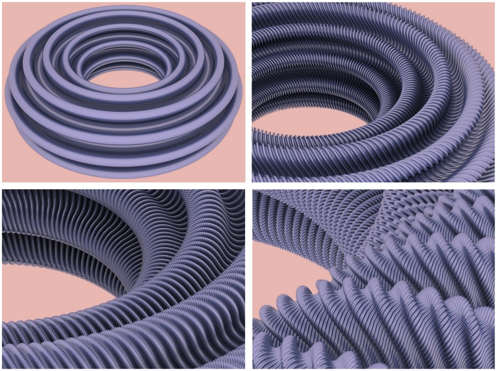
Cover image from professor Keenan Crane’s discrete differential geometry note.

Curvatures

Two fundamental mathematical approaches to describing a shape (space) $M$ involve addressing the following questions:

🤔 (Topological) How many holes are present in $M$?
🧐 (Geometrical) What is the curvature of $M$?

To address the first question, our space $M$ is considered solely in terms of its topology without any additional structure. For the second question, however, $M$ is assumed to be a Riemannian manifold—a smooth manifold equipped with a Riemannian metric, which is an inner product defined at each point. This category includes surfaces as we commonly understand them. This note aims to demystify Riemannian curvature, connecting it to the more familiar concept of curvature.

… Notoriously Difficult…

Riemannian curvature, a formidable name, frequently appears in literatures when digging into geometry. Fields Medalist Cédric Villani in his Optimal Transport said

“it is notoriously difficult, even for specialists, to get some understanding of its meaning.” (p.357)

Riemannian curvature is the father of curvatures we saw in our SGI tutorial and other curvatures. In the most abstract sense, Riemann curvature tensor is defined as a $(0,4)$ tensor field obtained by lowering the contravariant index of the $(1,3)$ tensor field defined as

\begin{aligned} R:\mathfrak{X}(M)\times \mathfrak{X}(M)\times\mathfrak{X}(M)&\to \mathfrak{X}(M)\\ (X,Y,Z)&\mapsto R(X, Y)Z:=\nabla_Y \nabla_X Z-\nabla_X \nabla_Y Z-\nabla_{[X, Y]} Z \end{aligned}

where $\nabla$ is the unique symmetric metric connection on $M$ called Levi-Civita connection and $[X,Y]$ is the Lie bracket of vector fields on $M$ …

So impenetrable 😵‍💫. Why bother using four vector fields to characterize the extent to which a space $M$ is curved?

To answer this question, we go to its opposite and try to get some of the common ways giving birth mathematical concepts.

What Does It Mean to Say Something Is Flat?

Flat Torus

A quote from prof. Crane’s discrete differential geometry note:

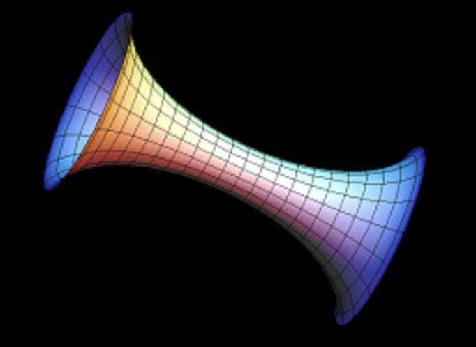
“It also helps to see pictures of surfaces with zero mean and Gaussian curvature. Zero-curvature surfaces are so well-studied in mathematics that they have special names. Surfaces with zero Gaussian curvature are called developable surfaces because they can be ‘developed’ or flattened out into the plane without any stretching or tearing. For instance, any piece of a cylinder is developable since one of the principal curvatures is zero:” (p.39)

Te following video continues with this cylinder example to show difficulties characterizing flatness. It examines the following question: how to use a piece of flat white paper to roll into a doughnut-shaped object (Torus) without distorting the length of the paper. That is, we are not allowed to use a piece of stretchable rubber to do this job.

Behind this video is this paper, where they used what Mikhael Gromov (my favorite mathematician) created when reviewing Nash embedding theorems to do the visualization.

This is part of an ongoing project. In fact, in an upcoming SIGGRAPH paper “Repulsive Shells” by Prof. Crane and others, more examples of isometric embeddings, including the flat torus, are discussed.

First definition of flatness

A Riemannian $n$-manifold is said to be flat if it is locally isometric to Euclidean space, that is, if every point has a neighborhood that is isometric (distance-preserving) to an open set in $\mathbb{R}^n$ with its Euclidean metric.

Example: flat torus

We denote the n-dimensional torus as $\mathbb{T}^n=\mathbb{S}^1\times \cdots\times \mathbb{S}^1$, regarded as the subset of $\mathbb{R}^{2n}$ defined by $(x^1)^2+(x^2)^2+\cdots+(x^{2n-1})^2+(x^{2n})^2=1$. The smooth covering map $X: \mathbb{R}^n \rightarrow \mathbb{T}^n$, defined by $X(u^1,\cdots,u^{n})=(\cos u^1,\sin u^1,\cdots,\cos u^n,\sin u^n)$, restricts to a smooth local parametrization on any sufficiently small open subset of $\mathbb{R}^n$, and the induced metric is equal to the Euclidean metric in $\left(u^i\right)$ coordinates, and therefore the induced metric on $\mathbb{T}^n$ is flat. This is called the Flat torus.

Parallel Transport

We still didn’t answer the question why we need four vector fields to characterize how curved a shape is. We will do this by using another useful tool in differential and discrete geometry to view flatness and thus curvedness. We follow John Lee’s Introduction to Riemannian Manifold for this section, first defining the Euclidean connection.

Consider a smooth curve $\gamma: I \rightarrow \mathbb{R}^n$, written in standard coordinates as $\gamma(t)=\left(\gamma^1(t), \ldots, \gamma^n(t)\right)$. Recall from calculus that its velocity is given by $\gamma'(t)=(\dot{\gamma}^1(t),\cdots,\dot{\gamma}^n(t))$ and its acceleration is given by $\gamma”(t)=(\ddot{\gamma}^1(t),\cdots,\ddot{\gamma}^n(t))$. A curve $\gamma$ in $\mathbb{R}^n$ is a straight line if and only if $\gamma^{\prime \prime}(t) \equiv 0$. Directional derivatives of scalar-valued functions are well understood in our calculus class. Analogs for vector-valued functions, or vector fields, on $\mathbb{R}^n$ can be computed using ordinary directional derivatives of component functions in standard coordinates. Given a vector $v$ tangent to $M$, we define the Euclidean directional derivative of vector field $Y$ in the direction $v$ by:

$$
\bar{\nabla}_v Y = \left.v(Y^1) \frac{\partial}{\partial x^1}\right|_p + \cdots + \left.v(Y^n) \frac{\partial}{\partial x^n}\right|_p,
$$

where for each $i$, $v(Y^i)$ is the result of applying the vector $v$ to the function $Y^i$:
$$
v(Y^i) = v^1 \frac{\partial Y^i(p)}{\partial x^1} + \cdots + v^n \frac{\partial Y^i(p)}{\partial x^n}.
$$

If $X$ is another vector field on $\mathbb{R}^n$, we obtain a new vector field $\bar{\nabla} _X Y$ by evaluating $\bar{\nabla} _{X_p} Y$ at each point:
$$
\bar{\nabla}_X Y = X(Y^1) \frac{\partial}{\partial x^1} + \cdots + X(Y^n) \frac{\partial}{\partial x^n}.
$$

This formula defines the Euclidean connection, generalizing the concept of directional derivatives to vector fields. This notion can be generalized to more abstract connections on $M$. When we say we parallel transport a tangent vector $v$ along a curve $\gamma$, we simply mean picking vectors for each point on the curve that are tagent to the curve and are parallel to each other at the same time. The mathematical way of saying vectors are parallel is to say the derivative of the vector field formed by them are zero (we have just defined the derivatives for vector field above). Let $T_pM$ denote the set of all vectors tangent to $M$ at point $p$, which forms a vector space.

Given a Riemannian 2-manifold $M$, here is one way to attempt to construct a parallel extension of a vector $z \in T_p M$: working in any smooth local coordinates $\left(x^1, x^2\right)$ centered at $p$, first parallel transport $z$ along the $x^1$-axis, and then parallel transport the resulting vectors along the coordinate lines parallel to the $x^2$-axis.

The result is a vector field $Z$ that, by construction, is parallel along every $x^2$ coordinate line and along the $x^1$-axis. The question is whether this vector field is parallel along $x^1$-coordinate lines other than the $x^1$-axis, or in other words, whether $\nabla_{\partial_1} Z \equiv 0$. Observe that $\nabla_{\partial_1} Z$ vanishes when $x^2=0$. If we could show that
$$
(*):\qquad \nabla_{\partial_2} \nabla_{\partial_1} Z=0
$$
then it would follow that $\nabla_{\partial_1} Z \equiv 0$, because the zero vector field is the unique parallel transport of zero along the $x^2$-curves. If we knew that $$ (**):\qquad
\nabla_{\partial_2} \nabla_{\partial_1} Z=\nabla_{\partial_1} \nabla_{\partial_2} Z,\text{ or } \nabla_{\partial_2} \nabla_{\partial_1} Z-\nabla_{\partial_1} \nabla_{\partial_2} Z = 0
$$
then $(\star)$ would follow immediately, because $\nabla_{\partial_2} Z=0$ everywhere by construction. We left showing it is true for $\bar{\nabla}$ as an exercise to readers [Hint: use our definition of Euclidean connection above and the calculus fact that $\partial_{xy}=\partial_{yx}$]. However, $(**)$ is not generally true for any connection. Lurking behind this noncommutativity is the fact that the sphere is “curved.”

For general vector fields $X$, $Y$, and $Z$, we can study $(**)$ as well. In fact, for $\bar{\nabla}$, computations easily lead to

$$\bar{\nabla}_X \bar{\nabla}_Y Z=\bar{\nabla}_X\left(Y\left(Z^k\right) \partial_k\right)=X Y\left(Z^k\right) \partial_k$$

and similarly $\bar{\nabla}_Y \bar{\nabla}_X Z=Y X\left(Z^k\right) \partial_k$. The difference between these two expressions is $\left(X Y\left(Z^k\right)-Y X\left(Z^k\right)\right) \partial_k=\bar{\nabla}{[X, Y]} Z$. Therefore, the following relation holds for $\nabla=\bar{\nabla}$:
$$
\nabla_X \nabla_Y Z-\nabla_Y \nabla_X Z=\nabla_{[X, Y]} Z .
$$

This condition is called flatness criterion.

Second definition of flatness

It can be shown that manifold $M$ is flat if and only if it satisfies flatness criterion! See Theorem 7.10 of Lee’s.

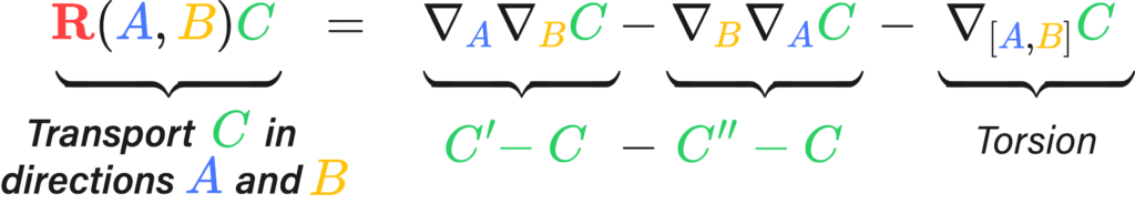
And finally, we comes back to our definition of Riemannian curvature $R$ we gave in the first section, which uses the difference between left-hand-side and right-hand-side of above condition to model the deviation of this flatness:

$$
R(X,Y)Z=\nabla_X \nabla_Y Z-\nabla_Y \nabla_X Z-\nabla_{[X, Y]} Z
$$

In our deformed mesh project, Dr. Nicholas Sharp showed a cool image of discrete parallel transport in his work with Yousuf Soliman and Keenan Crane.

Some “Downsides”

Now, four is good in the sense that it measures deviation from flatness, but it’s still computationally challenging to understand quantitatively. Besides, the Riemannian curvature tensor provides a lot of redundant information: there are a lot of symmetries of components of $Rm$, namely, the coefficients $R_{ijkl}$ such that

$$Rm = R_{ijkl} dx^1\otimes dx^j\otimes dx^k\otimes dx^l$$

The key symmetries are:

$ R_{ijkl} = -R_{jikl} $
$ R_{ijkl} = -R_{ijlk} $
$ R_{ijkl} = R_{klij} $
$ R_{ijkl} + R_{jkil} + R_{kijl} = 0 $

These symmetries show that knowing some of them allows to get many of the other components. They are good in that taking a glimpse at some of components gets us a full picture, but they are also bad in that these symmetries indicate that there is redundant information encoded in that tensor field.

More evidence is gathered. Interested readers may take a look: algebraic and differential Bianchi identities and Ricci identities

Alternatives

Preview: The following will be a brief review on some of the common notions of curvature, since understanding of some of them requires a solid base in Tensor algebra.

We seek to use simpler tensor fields to describe curvature. A natural way of doing this is to consider the trace of the Riemannian curvature. We recall from our linear algebra course that the trace of a linear operator $A$ is the sum of the diagonal elements of its matrix. This concept can be generalized to trace of tensor products, which can be thought of as the sum of diagonal elements of higher-dimensional matrix of tensor products. Ricci curvature $Rc$ is the trace of $Rm=R^\flat$ and scalar curvature $S$ is the trace of $Rc$.

Thanks to professor Oded Stein, we already learned in our first week SGI tutorial about principal curvature, mean curvature, and Gaussian curvature. Principal curvatures are the largest and smallest plane curve curvatures $\kappa_1,\kappa_2$ where curves are intersections of a surface and planes aligning with the (outward-pointing) normal vector at point $p$. This can be generalized to high-dimensional manifolds by observing that the argmin and argmax happen to be eigenvalues of shape operator $s$ and the fact that $h(v,v)=\langle sv,v\rangle$ and $|h(v,v)|$ is the curvature of a curve, where $h$ is the scalar second fundamental form. Mean curvature is simply the arithmetic mean of eigenvalues of $s$, namely $\frac{1}{2}(\kappa_1+\kappa_2)$ in the surface case; Gaussian curvature is the determinant of matrix of $s$, namely $\kappa_1\kappa_2$ in the surface case.

It turns out that Gaussian curvature is the bridge between those abstract Riemannian family $R,Rm, Rc, S$ and above curvatures that are more familiar to us. Gauss was so glad for finding that Gaussian curvature is a local isometry invariant that he named this discovery as Theorema Egregium, Latin for “Remarkable Theorem.” By this theorem, we can talk about Gaussian curvature of a manifold without worrying about where it is embedded. See here for a demo of Gauss map, which is used for his original definition of Gaussian curvature and the proof of the Theorema Egregium (see here for example). This theorem allows us to define the last curvature notion we’ll used: for a given two-dimensional plane $\Pi$ spanned by vectors $u,v\in T_pM$, the sectional curvature is defined as the Gaussian curvature of the $2$-dimensional submanifold $S_{\Pi} = \exp_p(\Pi\cap V)$ where $\exp_p$ is the exponential map and $V$ is the star-shaped subset of $T_pM$ for which $\exp_p$ restricts ot a diffeomorphism.

Geometric Interpretation of Ricci and Scalar Curvatures (Proposition 8.32 of Lee’s):

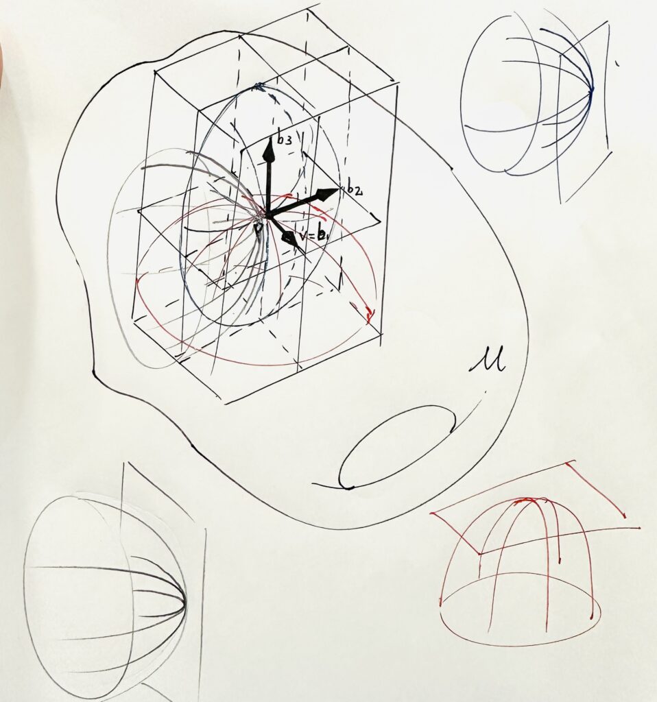
My attempt to visualize sectional curvatures.

Let $(M, g)$ be a Riemannian $n$-manifold and $p \in M$. Then

For every unit vector $v \in T_p M$, $Rc_p(v, v)$ is the sum of the sectional curvatures of the 2-planes spanned by $\left(v, b_2\right), \ldots, \left(v, b_n\right)$, where $\left(b_1, \ldots, b_n\right)$ is any orthonormal basis for $T_p M$ with $b_1 = v$.
The scalar curvature at $p$ is the sum of all sectional curvatures of the 2-planes spanned by ordered pairs of distinct basis vectors in any orthonormal basis.

General Relativity

Writing: Artur RB Boyago

Introduction: Artur studied physics before studying electrical engineering. Although curvatures of two dimensional objects are much easier to describe, physicists still need higher dimensional analogs to decipher spacetime.

I’d like to give a physicist’s perspective on this whole curvature thing, meaning I’ll flail my hands a lot. The best way I’ve come to understand Riemannian curvature is by the “area/angle deficit” approach.
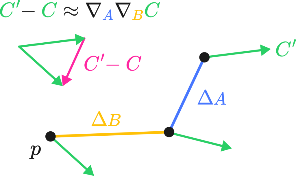
Imagine we had a little bit of a loop made up of two legs, $\Delta A$ and $ \Delta B$ at a starting point $p$. Were you to transport a little vector $C$ down these legs, keeping it as “straight as possible” in curved space. By the end of the two little legs, the vector $ C’ $ would have the same length but a slight rotation in comparison to $C$. We could, in fact, measure it by taking their difference vector (see the image on the left).

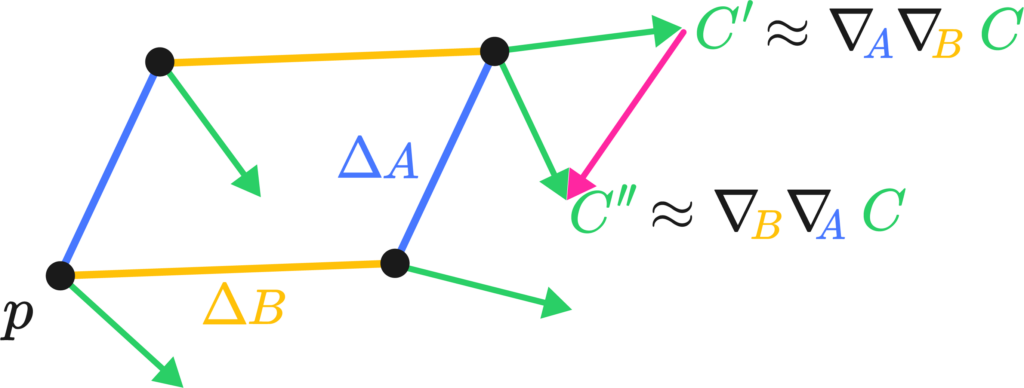
The difference vector is sort of the differential, or the change of the vector along the total path, which we may write down as $ \nabla_A \nabla_B C$, the two covariant derivatives applied to C along $A$ and $B$.
The critical bit of insight is that changing the order of the transport along $A$ and $B$ actually changes the result of said transport. That is, by walking north and then east, and walking east and then north, you end up at the same spot but with a different orientation.

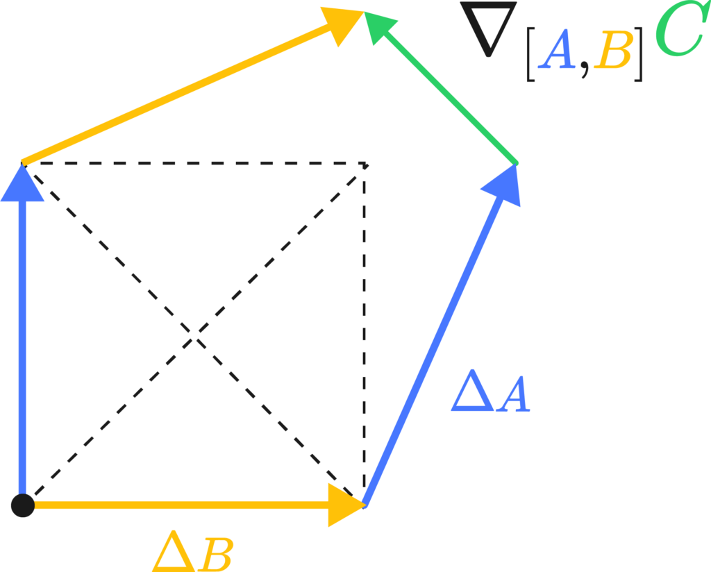
Torsion’s the same deal, but by walking north and then east, and walking east and then north you actually land in a different country.

The Riemann tensor is then actually a fairly simple creature. It has four different instructions in its indices, $R_{abc}^{\sigma}$,
and from the two pictures above we get three of them: Riemann measures the angle deficit or the degree of path-dependance of a region of space. This is the $R_{abc}$ bit

There’s one instruction left. It simply states in which direction we can measure the total difference vector produced by the path by means of a differential form, this closes up our $ R^{\sigma}{abc} $:

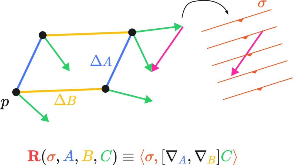
Funny how that works with electrons, they get all confused and get some charge out of frustration. Anyways, the properties of the Riemann tensor can be algebraically understood as these properties of “non-commutative transport” along paths in curved space. For example, the last two indices are naturally anticommutative, since it means the reversal of the direction of travel.

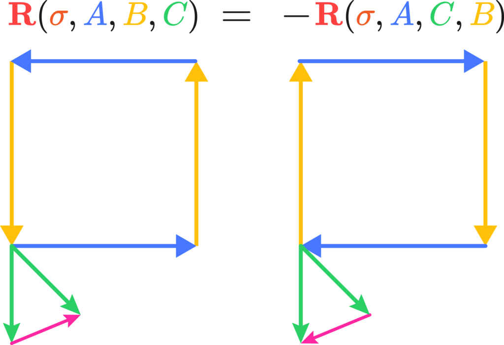
Similarly, it’s quite trivial that by switching the vector being transported and the covector doing the measuring also switches signs: $R^b_{acd} = -R^a_{bcd}, \; R^a_{bcd} = R^c_{dab}$
The Bianchi Identity is also a statement about what closes and what doesn’t, you can try drawing one that one pretty easily.
Now for the general relativity, this is quick; the Einstein tensor is the double dual of the Riemann tensor. It’s hard to see this in tensor calculus, but in geometric algebra it’s rather trivial; the Riemann tensor is a bivector to bivector mapping that produces rotation operators proportional to curvature, the Einstein tensor is a trivector to trivector volume that produces torque curvature operators proportionally to momentum-energy, or momenergy.
Torque curvature is an important quantity. The total amount of curvature for the Riemann tensor always vanishes because of some geometry, so if you tried to solve an equation for movement in spacetime you’d be out of luck.
But, you can look at the rotational deformation of a volume of space and how much it shrinks proportionally in some section of 3D space. The trick is, this rotational deformation is exactly equal to the content of momentum-energy, or momenergy, of the section.
\[\text{(Moment of rotation)} =
(e_a\wedge e_b \wedge e_c) \ R^{bc}_{ef} \ (dx_d\wedge dx_e\wedge dx_f) \approx 8\pi (\text{Momentum-energy})\]
This is usually written down as\[ \mathbf{G=8\pi T} \]Easy, ay?