Mentor:Dr. Karthik Gopinath
Volunteer Mentor: Kyle Onghai.
Fellows: Sergius Justus Nyah, Nicolas Pigadas, Mutiraj Laksanawisit
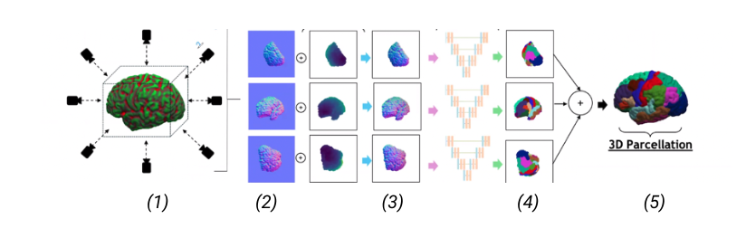
Picture 1: A high-level of the 2D projection descriptor pipeline we propose. (1) Extraction of multiple views and multiple descriptors from the 3D shape; (2) The extracted descriptors can be: normals, depth and curvature; (3) Input of the descriptors into a multi-view network; (4) Segmentation of the views (5) 3D reconstruction of the 3D segmented shape.
Abstract
Labeling brain surfaces is vital to many aspects of neuroscience and medicine, but to do so manually is laborious and time-consuming. An automated method would streamline the process, enabling more efficient analysis and interpretation of neuroimaging data. Such a task aligns with the longstanding inquiry in computer vision: is it more effective to use 3D shape representations or would 2D projection descriptor approaches yield better understanding of the shape? In this work, we explore the 2D approach of this question. We propose an automated end-to-end pipeline, structured into four main phases: selection of views for 2D projection extraction, rendering of the cortical mesh from multiple perspectives, segmentation of these projections and inverse rendering to map 2D segmentations back to 3D, integrating multiple views (Picture 1)
Definitions of Basic Project-Related Terms:
- Pseudo-Rendering: This is a process whereby a 3D model, such as a cortical mesh (in our case), is projected into 2D images from multiple perspectives. This process involves a transformation from the 3D coordinate space to the 2D image plane. The perspectives can be defined by a virtual camera’s position and orientation relative to the 3D model. The resulting 2D images retain depth information from the 3D model, hence bringing forth the perception of three-dimensionality.
- 2D Segmentation: 2D Segmentation is the process of dividing a 2D image into distinct regions based on pixel characteristics such as color, intensity, or texture. The segmentation method, which can include techniques like thresholding, clustering, watershed, and edge-based methods, determines how these regions are defined. For example, in an image of an airplane in the sky, one region might be the blue sky and another the white airplane. Similarly, an image of a chair could be segmented into regions representing the chair’s legs, seat, and backrest. Post-processing steps may be applied to refine these regions. The success of the segmentation can be evaluated using metrics like pixel accuracy, Intersection over Union (IoU), and Dice coefficient (a measure of the performance of Segmentation algorithms).
- Cortical Mesh: This is a 3D model that represents the outer surface of the brain (cerebral cortex), usually obtained from Magnetic Resonance Imaging data.
- Parcellation: This refers to the process of dividing cortical meshes, typically derived from brain imaging data, into distinct regions or parcels. These parcels often represent functionally or structurally distinct areas of the brain. Its purpose here is to simplify the analysis of brain imaging data by reducing the complexity of the data and focusing on regions of interest.
Initial Steps:
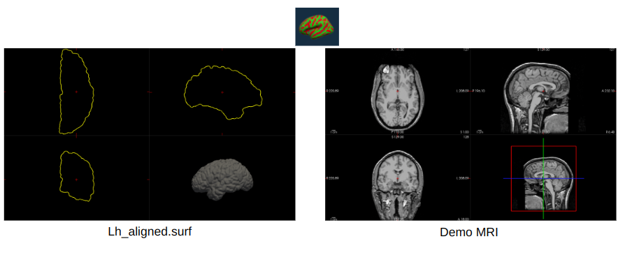
- Load and visualize Brain surfaces with FreeSurfer [Link]
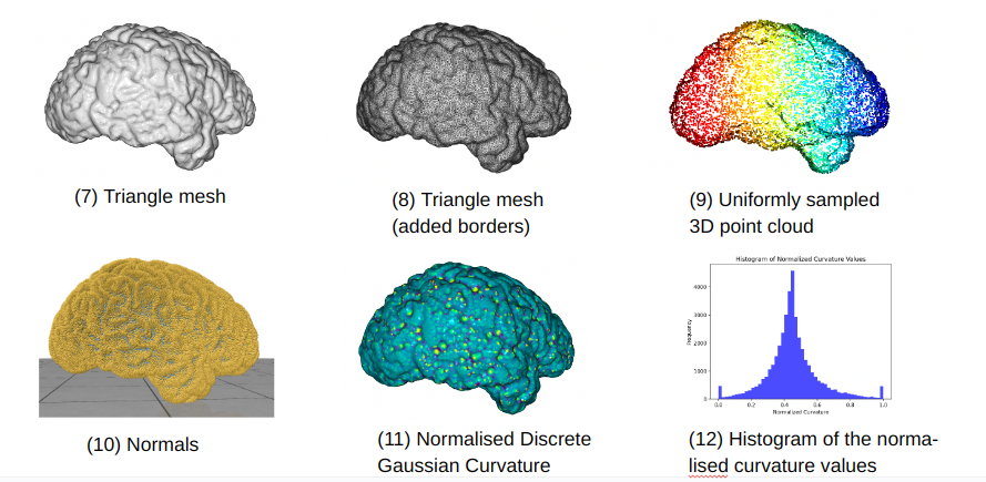
- Compute Normals, Curvature, and Point clouds from the Mesh surface
Method:
Selecting camera views to Extract 2D Images.
The selection of camera views is a critical step which involves determining the optimal perspectives from which to project the 3D cortical mesh onto 2D planes. Our goal here is to capture the most informative views that will facilitate accurate segmentation and subsequent inverse rendering.
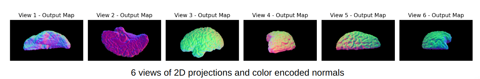
We will start adopting a systematic approach to select six canonical views: Front, Bottom, Top, Right, Back, and Left. These views are chosen to ensure comprehensive coverage of the cortical surface, capturing its intricate geometry from multiple angles.
The selection process begins by computing the intrinsic matrix for the camera, which is used to simulate the camera’s perspective. The intrinsic matrix is calculated using the following function in Python:
def compute_intmat(img_width, img_height):

    intmat = np.eye(3)

    # Fill the diagonal elements with appropriate values
    np.fill_diagonal(intmat, [-(img_width + img_height) / 1, -(img_width + img_height) / 1, 1])

    # Set the last column of the matrix for image centering
    intmat[:,-1] = [img_width / 2, img_height / 2, 1]

    return intmat
Next, we’ll create external transformation matrices to align the camera with the six predefined views. These matrices help us generate rays for ray casting, allowing us to simulate what the camera would see from each perspective. We’ll use the pinhole camera model to generate these rays.
def generate_maps(mesh, labels, intmat, extmat, img_width, img_height, rotation_matrices, recompute_normals):
    assert isinstance(mesh, o3d.t.geometry.TriangleMesh)
    assert isinstance(labels, np.ndarray) and labels.shape == (mesh.vertex.normals.shape[0],)
    assert isinstance(intmat, np.ndarray) and intmat.shape == (3, 3)
    assert isinstance(extmat, np.ndarray) and (extmat.shape == (1, 4, 4) or extmat.shape == (6, 4, 4))
    assert isinstance(img_width, int) and img_width > 0
    assert isinstance(img_height, int) and img_height > 0

    if recompute_normals:
        mesh.vertex.normals = mesh.vertex.normals@np.transpose(rotation_matrices[0][:3,:3].astype(np.float32))
        mesh.triangle.normals = mesh.triangle.normals@np.transpose(rotation_matrices[0][:3,:3].astype(np.float32))

    scene = o3d.t.geometry.RaycastingScene()
    scene.add_triangles(mesh)

    output_maps, labels_maps, ids_maps, vertex_maps = [], [], [], []

    for i in range(rotation_matrices.shape[0]):
        rays = scene.create_rays_pinhole(intmat, extmat[i], img_width, img_height)
        cast = scene.cast_rays(rays)
        ids_map = np.array(cast['primitive_ids'].numpy(), dtype=np.int32)
        ids_maps.append(ids_map)
        hit_map = np.array(cast['t_hit'].numpy(), dtype=np.float32)
        weights_map = np.array(cast['primitive_uvs'].numpy(), dtype=np.float32)
        label_ids = np.argmax(np.concatenate((weights_map, 1 - np.sum(weights_map, axis=2, keepdims=True)), axis=2), axis=2)

        normal_map = np.array(mesh.triangle.normals[ids_map.clip(0)].numpy(), dtype=np.float32)
        normal_map[ids_map == -1] = [0, 0, -1]
        normal_map[:, :, -1] = -normal_map[:, :, -1].clip(-1, 0)
        normal_map = normal_map * 0.5 + 0.5

        vertex_map = np.array(mesh.triangle.indices[ids_map.clip(0)].numpy(), dtype=np.int32)
        vertex_map[ids_map == -1] = [-1]
        vertex_maps.append(vertex_map)

        inverse_distance_map = 1 / hit_map
        coded_map_inv = normal_map * inverse_distance_map[:, :, None]
        output_map = (coded_map_inv - np.min(coded_map_inv)) / (np.max(coded_map_inv) - np.min(coded_map_inv))
        output_maps.append(output_map)

        labels_map = labels[vertex_map.clip(0)]
        labels_map[vertex_map == -1] = -1
        labels_map = labels_map[np.arange(labels_map.shape[0])[:, np.newaxis], np.arange(labels_map.shape[1]), label_ids]
        labels_map = labels_map.astype('float64')
        labels_maps.append(labels_map)

    return np.array(output_maps), np.array(labels_maps)
By casting rays from these six perspectives, we can project the entire cortical surface onto 2D planes, making sure we capture all the important features. This multi-view approach strengthens the segmentation process by reducing the chances of occlusions and giving us a more complete picture of the 3D structure.
The following images illustrate the six canonical views we used in our pipeline:
Now, We will accompany each 2D projection with annotations (ground truth).
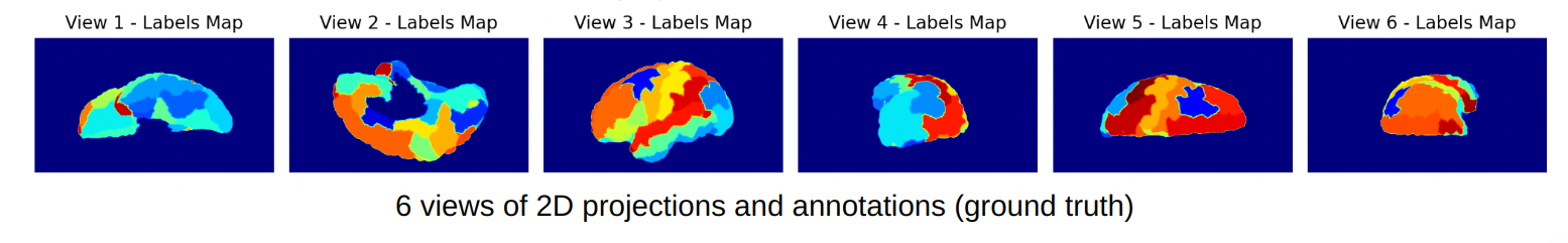
These views are crucial for the next steps in our pipeline, such as rendering, segmentation, and inverse rendering. By carefully choosing and using these perspectives, we improve both the accuracy and efficiency of the automated labeling process. The six camera positions ensure that every part of the cortical surface is captured, giving us a complete set of 2D projections that can be accurately mapped back to the 3D structure.
2D Projections: Annotations and Curvature
To continue, we take the 2D projections obtained from the six camera views and perform annotations and curvature calculations, which are essential for understanding the cortical surface’s geometry and features.
Process:
- Calculate the curvature of the cortical surface from the 2D projections, which helps in identifying important features and understanding the surface’s geometry.
- Annotate the 2D projections with relevant labels, such as different brain regions or anatomical landmarks.
- Use these annotations to the CNN (As seen below) for automated labeling.
Code:
# Compute per-face curvature using gpytoolbox (angle defect)
curvature = gpy.angle_defect(vertices, faces)


# Debugging: Print raw curvature values
print("Raw Curvature Values:")
print(curvature)
print("Curvature min:", np.min(curvature))
print("Curvature max:", np.max(curvature))


# Percentile-based normalization
lower_percentile = np.percentile(curvature, 1)
upper_percentile = np.percentile(curvature, 99)


# Clipping the curvature values to the 1st and 99th percentiles to diminish the effect of outliers
curvature_clipped = np.clip(curvature, lower_percentile, upper_percentile)


# Normalize the clipped curvature values between 0 and 1
curvature_normalized = (curvature_clipped - lower_percentile) / (upper_percentile - lower_percentile)


# Debugging: Print normalized curvature values
print("Normalized Curvature Values:")
print(curvature_normalized)


# Select color map
color_map = plt.get_cmap('viridis')
curvature_colors = color_map(curvature_normalized)[:, :3] # Ignore alpha channel


# Create Open3D mesh
mesh = o3d.geometry.TriangleMesh()
mesh.vertices = o3d.utility.Vector3dVector(vertices)
mesh.triangles = o3d.utility.Vector3iVector(faces)
mesh.vertex_colors = o3d.utility.Vector3dVector(curvature_colors) # Apply colors to vertices


# Compute normals to improve lighting in visualization
mesh.compute_vertex_normals()


# Visualize the mesh with curvature coloring
o3d.visualization.draw_geometries([mesh], window_name='Mesh with Curvature Colors')


# Visualize the normalized curvature values as a histogram
plt.figure()
plt.hist(curvature_normalized, bins=50, color='blue', alpha=0.7)
plt.title("Histogram of Normalized Curvature Values")
plt.xlabel("Normalized Curvature")
plt.ylabel("Frequency")
plt.show()
Result (As seen also in (2) above):
Training the multi-view CNN
Now we use the annotated 2D projections to train a multi-view Convolutional Neural Network (CNN). This multi-view CNN leverages the different perspectives to improve the accuracy of the labeling process.
Process:
- Data Preparation:
- Prepare the annotated 2D projections as input data for the CNN.
- Split the data into training, validation, and test sets.
import os
import nibabel as nib
import torch
from torch.utils.data import Dataset, DataLoader

def load_data(data_dir):

    data = []
    labels = []

    for subject_dir in os.listdir(data_dir):
        surf_dir = os.path.join(data_dir, subject_dir, 'surf')
        label_dir = os.path.join(data_dir, subject_dir, 'label')

        if os.path.isdir(surf_dir) and os.path.isdir(label_dir):
            # Load surface data
            surf_file = os.path.join(surf_dir, 'lh_aligned.surf')
            if os.path.exists(surf_file):
                surf_data = nib.freesurfer.read_geometry(surf_file)[0]
                data.append(surf_data)

            # Load label data
            label_file = os.path.join(label_dir, 'lh.annot')
            if os.path.exists(label_file):
                label_data = nib.freesurfer.read_annot(label_file)[0]
                labels.append(label_data)

    return np.array(data), np.array(labels)


# Load actual data
train_data, train_labels = load_data('/home/sergy/cortical-mesh-parcellation/10brainsurfaces (1)')
val_data, val_labels = load_data('/home/sergy/cortical-mesh-parcellation/10brainsurfaces (1)')


# Convert data to PyTorch tensors
train_data = torch.tensor(train_data, dtype=torch.float32)
train_labels = torch.tensor(train_labels, dtype=torch.long)
val_data = torch.tensor(val_data, dtype=torch.float32)
val_labels = torch.tensor(val_labels, dtype=torch.long)


# Define custom dataset class
class ExampleDataset(Dataset):
    def __init__(self, data, labels):
        self.data = data
        self.labels = labels

    def __len__(self):
        return len(self.data)

    def __getitem__(self, index):
        return self.data[index], self.labels[index]


# Create DataLoader for training and validation data
train_dataset = ExampleDataset(train_data, train_labels)
val_dataset = ExampleDataset(val_data, val_labels)

train_loader = DataLoader(train_dataset, batch_size=32, shuffle=True)
val_loader = DataLoader(val_dataset, batch_size=32, shuffle=False)2. Model Architecture:
- Design a CNN architecture that can handle multi-view inputs.
- Use techniques like data augmentation to improve the model’s robustness.
from trainCNN import MultiViewCNN
import torch.nn as nn

# Initialize the model
model = MultiViewCNN()

# Define the loss function and optimizer
criterion = nn.CrossEntropyLoss()
optimizer = torch.optim.Adam(model.parameters(), lr=0.001)
3. Training the CNN:
- Train the CNN using the prepared data.
- Monitor the training process using metrics like accuracy and loss.
# Training loop
for epoch in range(5):  # 5 epochs
    model.train()
    for i, (inputs, labels) in enumerate(train_loader):
        optimizer.zero_grad()
        outputs = model(inputs)
        loss = criterion(outputs, labels)
        loss.backward()
        optimizer.step()

        if i % 100 == 0:
            print(f"Epoch [{epoch+1}/5], Step [{i+1}/{len(train_loader)}], Loss: {loss.item():.4f}")

    # Validation loop
    model.eval()
    val_loss = 0.0
    with torch.no_grad():
        for inputs, labels in val_loader:
            outputs = model(inputs)
            loss = criterion(outputs, labels)
            val_loss += loss.item()

    val_loss /= len(val_loader)
    print(f"Validation Loss after Epoch [{epoch+1}/5]: {val_loss:.4f}")
Training result:
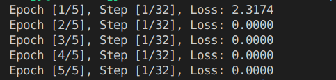
Analysis of Training Results:
Initial Loss: In the first epoch, the initial loss is 2.3174. This indicates that the model is starting to learn from the data, but there is still a significant difference between the predicted and actual labels.
Subsequent Epochs: From the second epoch onwards, the loss drops to 0.0000. This suggests that the model has quickly learned to minimize the loss and make accurate predictions.
3D Reconstruction: Annotations and Curvature:
To conclude, we will map the 2D annotations and curvature back to the 3D structure, which provides a comprehensive view of the cortical surface with detailed annotations and curvature information. We can divide this into 3 steps;
- Mapping Annotations:
Firstly, we will map the annotations predicted by the Multi-View CNN back to the 3D cortical surface, which involves projecting the 2D annotations onto the 3D mesh.
import numpy as np
def map_annotations_to_3d(annotations_2d, vertices, faces):
    # Initialize a 3D array to store the annotations
    annotations_3d = np.zeros(vertices.shape[0])
    # Iterate over each face and map the 2D annotations to the 3D vertices
    for i, face in enumerate(faces):
        for vertex in face:
            annotations_3d[vertex] = annotations_2d[i]
    return annotations_3d
# Example usage
annotations_2d = np.random.randint(0, 10, size=(faces.shape[0],))  # Replace with actual 2D annotations
annotations_3d = map_annotations_to_3d(annotations_2d, vertices, faces)
2. Mapping Curvature:
We then map the calculated curvature values from the 2D projections back to the 3D surface. This will help us in visualizing the curvature on the 3D model.
def map_curvature_to_3d(curvature_2d, vertices, faces):
    # Initialize a 3D array to store the curvature values
    curvature_3d = np.zeros(vertices.shape[0])

    # Iterate over each face and map the 2D curvature to the 3D vertices
    for i, face in enumerate(faces):
        for vertex in face:
            curvature_3d[vertex] = curvature_2d[i]

    return curvature_3d

# Define vertices and faces
vertices = np.array([[0, 0, 0], [1, 0, 0], [1, 1, 0], [0, 1, 0]])
faces = np.array([[0, 1, 2], [0, 2, 3]])
3. Integration and Visualization:
Finally, we will integrate the annotations and curvature into a single 3D model and use a visualization tool (Polyscope, in this case) to display the final annotated and curved 3D structure.
# Load annotations and curvature data
annotations_path = '10brainsurfaces (1)/100206/label/lh.annot'
curvature_path = 'curvature_array.npy'
annotations_3d = nib.freesurfer.read_annot(annotations_path)[0]
curvature_3d = np.load(curvature_path)
# Ensure curvature_3d has the correct shape
if curvature_3d.shape[0] != vertices.shape[0]:
    curvature_3d = curvature_3d[:vertices.shape[0]]
# Initialize Polyscope
ps.init()

# Register the 3D mesh with Polyscope
mesh = ps.register_surface_mesh("annotated_brain", vertices, faces)
# Add the annotations and curvature as scalar quantities
mesh.add_scalar_quantity("annotations", annotations_3d, defined_on="vertices", cmap="viridis")
mesh.add_scalar_quantity("curvature", curvature_3d, defined_on="vertices", cmap="coolwarm")
# Show the visualization
ps.show()
Final Results from Annotations and Mappings:
Our pipeline successfully achieved its goals:
- The trainCNN script trained the MultiViewCNN model and saved the state dictionary.
- The projections.py script visualized the cortical mesh with annotations and curvature, as seen below
- The trained model extracted features from the 2D projections, enhancing our understanding of the cortical surface.
- Our goal of Pseudo Rendering was achieved.
Figure 1: Front view of brain section with labeled annotations:
Figure 2: Back view of brain section with labeled annotations:
To conclude this long post, permit us discuss the practical use-scopes of Pseudo rendering, across diverse feilds in Science, healthcare, and Research:
- Pseudo-rendering enhances the visualization of complex anatomical structures, aiding in better diagnosis and treatment planning by providing detailed 3D models of organs and tissues.
- Enables efficient analysis of 3D data by generating 2D projections from multiple camera angles, like in the case of cortical mesh parcellation.
- Reduces computational resources required for rendering complex 3D models, making the process less resource-intensive.
- Supports interactive exploration of 3D models, allowing users to manipulate 2D projections to explore different views and perspectives.
Closing Remarks:
At this point, we would like to express our gratitude to our amazing mentor, Dr. Karthik Gopinath, and volunteer mentor, Kyle Onghai, for their unwavering support and guidance throughout the project. Their effective guidance enabled us to rapidly develop our ideas and foster a deep passion for the project. We look forward to continuing our work on this brilliant research idea as soon as possible.
Thank you for reading this far! 🎉
Long Live the SGI!