
By Juan Parra, Kimberly Herrera, and Eleanor Wiesler
Project mentors: Silvia Sellán, Noam Aigerman
Introduction
Given a surface we can represent it moving along certain trajectory in space by a swept area or swept volume. It’s a good idea to take this approach to model 3D shapes or to detect a collision of the shape with another shape in its environment. There are several algorithms in the literature that address the construction of the surface of a swept volume in space, each taking their respective assumptions on the surface and the trajectory.
In our project we trained neural networks to predict the sweeping of a surface, and attempted to find the best representation of a neural network that deals with discontinuities that appear in the process.
Using Signed-Distance Functions to Model Shape Sweeping
By a swept volume we mean the trajectory that a solid moving through space made. The importance of representing a swept volume can go from art modeling to collision detection in robotics. We can model the swept volume of the solid motion as a surface in 3D. The goal of this project is to train neural networks to learn swept volumes, and so we conducted the experiments of this study using 2D shapes swept across a trajectory in the coordinate plane and evaluated resulting swept area. To study the trajectory or “sweeping” of these shapes, we used Signed Distance Functions (SDFs).
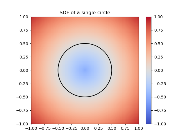
Figure 1: SDF of a single circle
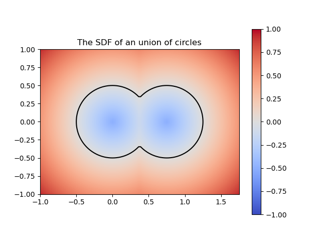
Figure 2: SDF of a union of circles
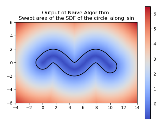
Finite Stamping
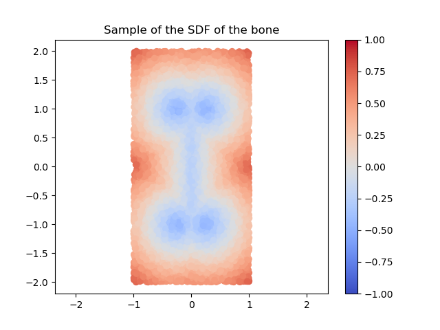
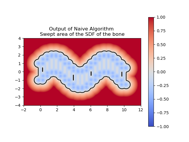
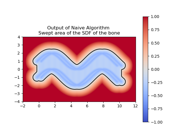
(a) 20 times
(b) 100 times
Learning Swept SDFs with Neural Networks
How to use a NN for SDFs
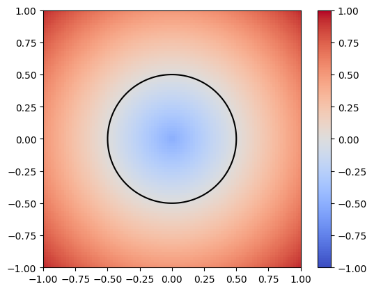
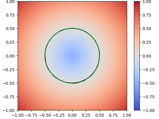
A neural network is just a function with many parameters; we can tweak these parameters to best approximate an SDF. To train the network, we first sample random points from the circle and compute their actual SDF values. The network’s goal is to predict these SDF values. By comparing the predicted values to the actual values using a loss function, the network can adjust its parameters to reduce the error. This adjustment is typically done through gradient descent, which iteratively refines the network’s parameters to minimize the loss. After training, we visualize the results to assess how well the neural network has learned to approximate the SDF. In the image below, the green represents the prediction for the circle by the neural network.
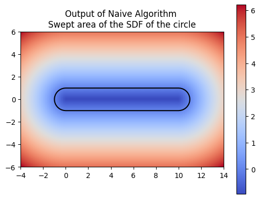
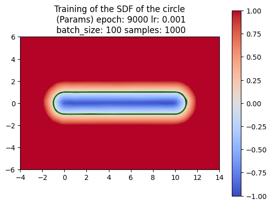
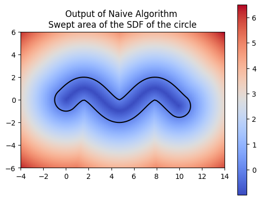
For computing a swept area, the neural network needs to approximate the union of multiple SDFs that together represent the swept area. Computing the swept area involves shifting the SDF along the trajectory at various points in time and then taking the union of all these SDFs. Once we understood how to compute the swept area ourselves, we had the neural network attempt the same. The following images show the results of our manual computation, which we refer to as the naive algorithm, for the sweeping of the circle along a horizontal path in comparison to the computation produced by the neural network. Similarly, the green represents the prediction for the swept area by the neural network.
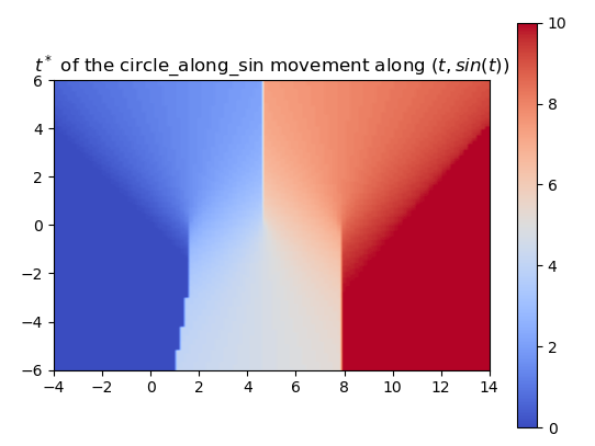
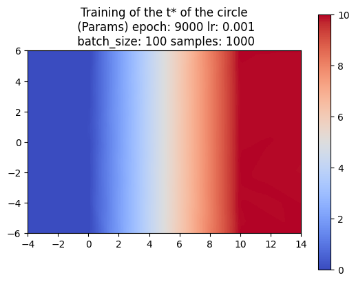
So far, we’ve trained the neural network to compute the SDF values for each point in a 2D grid. Now, since we are sweeping a shape over time, we want the network to return the times corresponding to these SDF values. We call these times t*. With the same shape and trajectory as above, the network has little issue doing this.
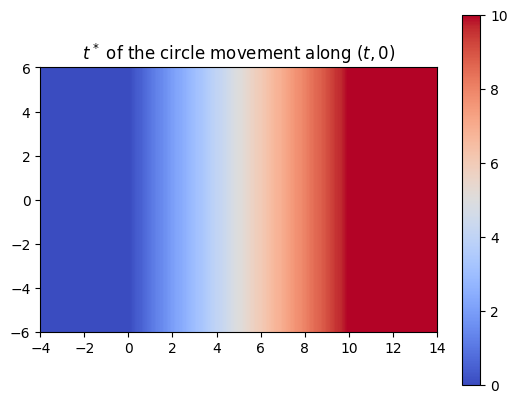
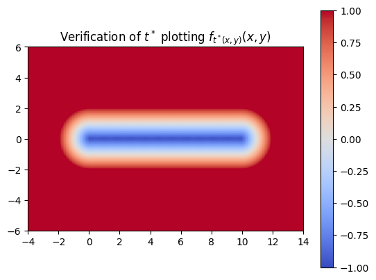
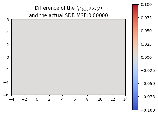
We also made sure that the t*‘s that we computed were producing the correct SDF of the swept area.
NN Difficulties detecting discontinuities
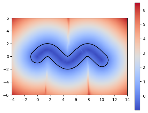
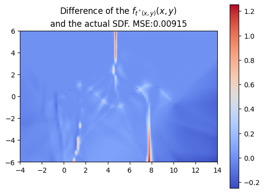
Using a more complex trajectory, such as a sine wave, introduces some challenges. While the neural network performs well in predicting the t* values, issues arise when computing the SDF with respect to these times. Specifically, the resulting SDF shows three lines emerging from the peaks and troughs of the curve. We can see this even more through the MSE plot.
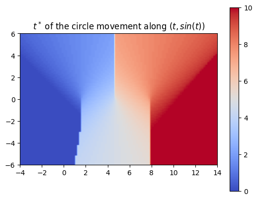
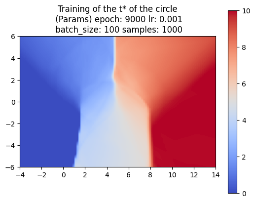
The left image shows the sweeping of the circle using the t* values computed by the neural network.
These challenges become even more apparent when using shapes with sharper edges such as a square. Because of this, we decided to work on optimizing the neural network architecture.
Adjusting Our Neural Network Architecture
Changing Our Activation Function
Every neural network has a defined activation function. In the case of our preliminary neural network experiments above, the specified activation function was a Rectified Linear Unit (ReLU). Despite this, we did not achieve the most desirable outcome of minimal error in the predicted swept SDF versus the naive algorithm swept SDF. Specifically, we observed errors at sites of discontinuity, where there were changes in sign, for example.
In an attempt to improve neural network performance, we decided to experiment with different activation functions by altering our neural network architecture. Below, we present their corresponding results when used for swept SDF prediction.
ReLU Function (Rectified Linear Unit Function)
Logistic Sigmoid Function
Hyperbolic Tangent Function