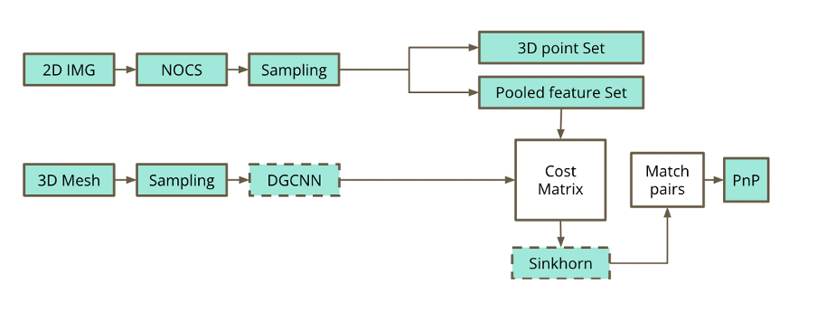
Image 1: Our proposed solution’s pipeline, credits to our -always supportive- mentors, Saleh Mahdi and Dani Velikova!
Introduction
Our project aims to enhance Optimal Transport (OT) solvers by incorporating Graph Neural Networks (GNNs) to address the lack of geometric consistency in feature matching. The main motivation of our study is that a lot of real objects are symmetric and thus impose ambiguity. Traditional OT approaches focus on similarity measures and often neglect important neighboring information in geometric settings, proper in computer vision or graphics problems, resulting in the production of huge noise in pose estimation tasks. To tackle this problem, we hypothetize that when the object is symmetric, there are many correct matches of points around its symmetric axis and we can leverage this fact via Optimal Transport and Graph Learning.
To this end, we propose the pipeline in image 1. On a high level, we extract a 3D point cloud of an object from a 2D scene using the Normalized Object Coordinate Space (NOCs) pipeline [1], downsample the points and pool the features/NOCs embeddings of the removed points into the representative remaining points. Concurrently, we run DGCNN on the 3D ground truth mesh of the object and create a graph; this model is used as a 3D encoder [2]. We combine the aforementioned embeddings into the cost matrix used by the Sinkhorn algorithm [3], which attempts to match the points of the point cloud produced by the NOCs map with the nodes of the graph produced by the DGCNN and then to provide a symmetry estimation. We extend the differentiable Sinkhorn solver to yield one-to-many solutions; a modification we make to fully capture the symmetry of a texture-less object. In the final step, we match pairs of points and pixels and perform symmetric pose estimation via Perspective-n-Point. In this post, we study one part of our proposed pipeline, the extended NOCs, from the 2D image analysis to the extraction of the 3D point set and the pooled feature set.
Extended NOCs pipeline
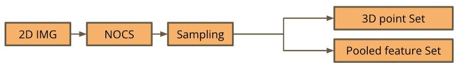
Image 2: The part of the pipeline we will study in this post: Generating a 3D point cloud of a shape from a chosen 2D scene and downsampling its points. We pool the features of the removed points into remaining (seed) points.
The NOCs pipeline extracts the NOCs map and provides size and pose estimation for each object in the scene. The NOCs map encodes via colours the prediction of the normalized 3D coordinates of the target objects’ surfaces within a bounded unit cube. We extend the NOCs pipeline to create a 3D point cloud of the target object using the extracted NOCs map. We then downsample the point cloud, by fragmenting it using the Farthest Point Sampling (FPS) algorithm and only keeping the resulting seed points. In order to fully encapsulate the information extracted by the NOCs pipeline, we pool the embeddings of the nodes of each fragment into the seed points, by averaging them. This enables our pipeline to leverage the features of the target object’s 2D partial view in its scene.
Data
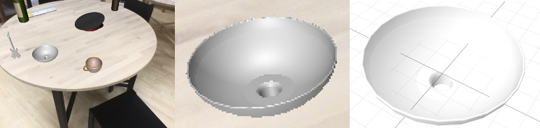
Images 3, 4, 5: (3) The scene of the selected symmetric and texture-less object. (4) The object in the scene zoomed in. (5) The ground truth of the object, i.e. its exact 3D model.
In order to test our hypothesis, we use an object that is not only symmetric, but also texture-less and pattern-free. The specifications of the object we use are the following:
- Dataset: camera, val data
- Scene: bundle 00009, scene 0001
- Object ids: 02880940, fc77ad0828db2caa533e44d90297dd6e
- Link to download: https://github.com/sahithchada/NOCS_PyTorch?tab=readme-ov-file
Extended NOCs pipeline: steps visualised
In this section we visually examine each part of the pipeline and how it processes the target shape. First, we get a 2D image of a 3D scene, which is the input of the NOCs pipeline:
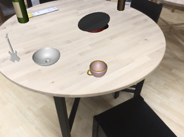
Image 6: The 3D scene to be analyzed.
Running the NOCs pipeline on it, we get the pose and size estimation, as well as the NOCs map for every object in the scene:
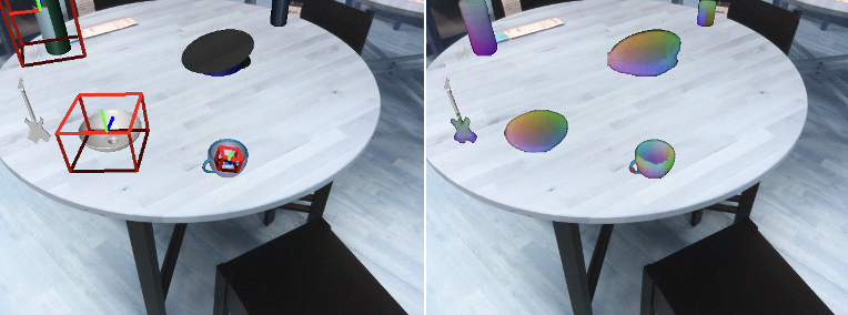
Image 7, 8: (7) Pose and size estimation of the objects in the scene. (8) NOCs maps of the objects.
The color encodings in the NOCs map encode the prediction of the normalized 3D coordinates of the target objects’ surfaces, within a bounded a unit cube. We leverage this prediction to reconstruct the 3D point cloud of our target shape, from its 2D representation in the scene. We used a statistical outlier removal method to refine the point cloud and remove noisy points. We got the following result:
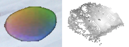
Images 9, 10: (9) The 2D NOCs map of the object. (10) The 3D point cloud reconstruction of the 2D NOCs map of the target object.
The extracted 3D point cloud of the target object is then fragmented using the Farthest Point Sampling (FPS) algorithm and the seed (center/representative) points of each fragment are also calculated.
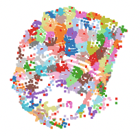
Image 11: The fragmented point cloud of the target object. Each fragment contains its corresponding seed point.
The Sinkhorn algorithm part of our project requires a lot less data points for an optimized performance. Thus, we downsample the 3D point cloud, by only keeping the seed points. In order to capture the information extracted by the NOCs pipeline, we pool the embeddings of the removed features into their corresponding seed points via averaging:
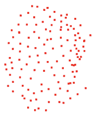
Image 12: The 3D seed point cloud. Into each seed point, we have pooled the embeddings of the removed points of their corresponding fragment.
An overview of each step and the visualised result can be seen below:
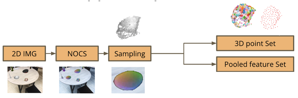
Image 13: The scene and object’s visualisation across every step of the pipeline.
Conclusion
In this study, we discussed the information extraction of a 3D object from a 2D scene. In our case, we examined the case of a symmetric object. We downsampled the resulting 3D point cloud in order for it to be effectively handled by later stages of the pipeline, but we made share to encapsulate the features of the removed points via pooling. It will be very interesting to see how every part of the pipeline comes together to predict symmetry!
At this point, I would like to thank our mentors Mahdi Saleh and Dani Velikova, as well as Matheus Araujo for their continuous support and understanding! I started as a complete beginner to these computer vision tasks, but I feel much more confident and intrigued by this domain!
Implementation
repo: https://github.com/NIcolasp14/MIT_SGI-Extended_NOCs/tree/main
References
[1] He Wang, Srinath Sridhar, Jingwei Huang, Julien Valentin, Shuran Song, and Leonidas J. Guibas. Normalized object coordinate space for category-level 6d object pose and size estimation, 2019.
[2] Yue Wang, Yongbin Sun, Ziwei Liu, Sanjay E. Sarma, Michael M. Bronstein, and Justin M. Solomon. Dynamic graph cnn for learning on point clouds, 2019.
[3] Paul-Edouard Sarlin, Daniel DeTone, Tomasz Malisiewicz, and Andrew Rabinovich. Superglue: Learning feature matching with graph neural networks. CoRR, abs/1911.11763, 2019.