Mentor: Amir Vaxman
Volunteer: Alberto Tono
Fellows: Mutiraj Laksanawisit, Diana Aldana Moreno, Anthony Hong
Our task is to fit closed and watertight surfaces to point clouds that might have a lot of noise and inconsistent outliers. There are many papers like this, where we will explore a modest variation on the problem: we will allow the system to modify the input point clouds in a controlled manner, where the modification will be gradually scaled back until the method fits to the original point clouds. The point of this experiment is to check whether such modification is beneficial for both accuracy and training time.
Regular Point-Cloud Fitting
A point clouds is an unordered set of 3D points: \(\mathscr{P}=\left\{x_i, y_i, z_i\right\}\), where \(0<i\leq N\) for some size \(N\). These points can be assumed to be accompanied by normals \(n_i\) (as unit vectors associated to each points). An \emph{implicit} surface reconstruction tries to fit a function \(f(x,y,z)\) to every point in space, such that its zero set
$$
S = f^{-1}(0)=\left\{(x,y,z) | f(x,y,z)=0\right\}
$$
represents the surface.
We usually train \(f\) to be a signed distance function (SDF) \(\mathbb{R}^3\rightarrow\mathbb{R}\) from the zero set. That is, to minimize the loss:
$$
f = \text{argmin}\left(\lambda_{p}E_p+\lambda_{n}E_n+\lambda_{s}E_s\right)
$$
where
\begin{align}
E_p &= \sum_{i=0}^N{|f(x_i,y_i,z_i)|^2}\\
E_n &= \sum_{i=0}^N{|\nabla f(x_i,y_i,z_i)-n_i|^2}\\
E_s &= \sum_{j=0}^Q{||\nabla f(x_j,y_j,z_j)|-1|^2}
\end{align}
Loss term \(E_p\) is for the zero-set fitting. Loss term \(E_n\) is for the normal fitting, and term \(E_s\) is for regulating \(f\) to be an SDF; it is trained on a randomly sampled set \(\mathscr{Q}=\left(x_j,y_j,z_j\right)\) (of size \(Q=|\mathscr{Q}|\)) in the bounding box of the object, that gets replaced every few iterations. The bounding box should be a bit bigger, say cover %20 more in each axis, to allow for enough empty space around the object.
Reconstruction Results
We extracted meshes from this repository and apply Poisson disc sampling with point-number parameter set at 1000 (but note that the resulted sampled points are not 1000; see the table below) on MeshLab2023.12. We then standardize the grids and normalize the normals (the xyz file with normals does not give normals in this version of MeshLab so we need to an extra step of normalization). Then we ran the learning procedure on these point clouds to fit an sdf with 500 epochs and other parameters shown below.
net = train_sdf_net(standardized_points, normals, epochs=500, batch_size=N,
learning_rate=0.01, lambda_p=1.0, lambda_n=1.5, lambda_s=0, neuron_factor=4)
We then plots the results (the neural netwok, the poitclouds and normals) and registered isosurfaces as meshes on polyscope and used slice planes to see how good are the fits. Check the table below.
| Nefertiti | Homer | Kitten | |
| Original meshes |  |  | |
| Vertices of sample | 1422 | 1441 | 1449 |
| Reconstructions |  |  |  |
| slice 1 |  |  |  |
| slice 2 |  |  |  |
| slice 3 |  |  |  |
| slice 4 |  |  |  |
| slice 5 |  |  |  |
| slice 6 |  |  |  |
Ablation Test
There are several parameters and methods we can play around. Basically, we did not aim to prove for some “optimal” set of parameters. Our approach is very experimental: we tried different set of parameters (learning rate, batch size, epoch number, and weights of each energy term) and see how good is the fit for each time we changed the set. If the results look good then the set is good, and the set we chose is included in the last subsection. We used the ReLU activation function and the results are generally good. We also tried tanh, which gives smoother reconstructed surfaces.
Adversarial Point Cloud Fitting
First try to randomly add noise to the point cloud of several levels, and try to fit again. You will see that the system probably performs quite poorly. Do so by adding a \(\epsilon_i\) to each point \((x_i,y_i,z_i)\) of a small Gaussian distribution. Test the result, and visualize it to several variances of noise.
We’ll next reach the point of the project, which is to learn an adversarial noise. We will add another module \(\phi\) that connects between the input and the network, where:
$$
\phi(x,y,z) = (\delta, p)
$$
\(\phi\) outputs a neural field \(\delta:\mathbb{R}^3\rightarrow \mathbb{R}^3\), that serves as a perturbation of the point clouds, and another neural field \(p:\mathbb{R}^3\rightarrow [0,1]\) that serves as the confidence measure of each point. Both are fields; that is they are defined ambiently in \(\mathbb{R}^3\), but we’ll use their sampling on the points \(\mathscr{P}_i\). Note that \(f\) is the same way!
The actual input to \(f\) is then \((x,y, z)+\delta\), where we extend the network to also receive \(p\). We then use the following augmented loss:
$$
f = \text{argmin}\left(\lambda_{p}\overline{E}_p+\lambda_{n}\overline{E}_n+\lambda_{s}\overline{E}_s +\lambda_d E_d + \lambda_v E_v + \lambda_p E_p\right),
$$
where
\begin{align}
E_d &= \sum_{i=0}^N{|\delta_i|^2}\\
E_v &= \sum_{i=0}^N{|\nabla \delta_i|^2}\\
E_p &= -\sum_{i=0}^N{log(p_i)}.
\end{align}
\(E_d\) regulates the magnitude of \(\delta\); it is zero if we try to adhere to the original point cloud. \(E_v\) regulates the smoothness of \(\delta\) in space, and \(E_p\) encourages the point cloud to trust the original points more, according to their confidences (it’s perfectly \(0\) when all \(p_i=1\). We use \(\delta_i=\delta(x_i,y_i,z_i)\) and similarly for \(p_i\).
The original losses are also modified according to \(\delta\) and \(p\): consider \(\overline{f} = f((x,y,z)+\delta)\), then:
\begin{align}
\overline{E}_p &= \sum_{i=0}^N{p_i|\overline{f}(x_i,y_i,z_i)|^2}\\
\overline{E}_n &= \sum_{i=0}^N{p_i|\nabla \overline{f}(x_i,y_i,z_i)-n_i|^2}\\
\overline{E}_s &= \sum_{j=0}^Q{||\nabla \overline{f}(x_j,y_j,z_j)|-1|^2}
\end{align}
By controlling the learnable \(\delta\) and \(p\), we aim to achieve a better loss; that essentially means smoothing the points and trusting those that are less noisy. This should result is quicker fitting, but less accuracy. We then, gradually with the iterations, try to increase \(\lambda_{d,v,p}\) more and more so to subdue \(\delta\) and trust the original point cloud more and more.
Reconstruction Results
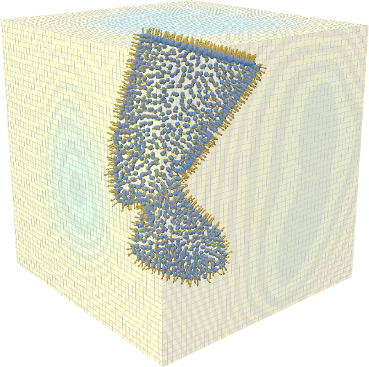
We use a network with a higher capacity to represent the perturbations \(\delta\) and the confidence probability \(p\). Specifically, we define a \(2\)-hidden layer ReLU MLP with sine for the first activation layer. This allows to represent high frequency details necessary to approximate the noise \(\delta\).
During the experiments, we notice that the parameters \(\lambda_d\), \(\lambda_v\), and \(\lambda_p\) have different behaviors over the resulting loss. The term \(E_d\) converges easily, so the value for \(\lambda_d\) is chosen to be small. On the other hand, the loss \(E_v\) that regulates smoothness is harder to fit so we choose a bigger \(\lambda_v\). Finally, the term \(E_p\) is the most sensitive one since it is defined as a sum of logarithms, meaning that small coordinates of \(p\) may lead to \(\texttt{inf}\) problems. For this term, a not so big, not so small value must be chosen, so as to have a confidence parameter near \(1\) and still converge.
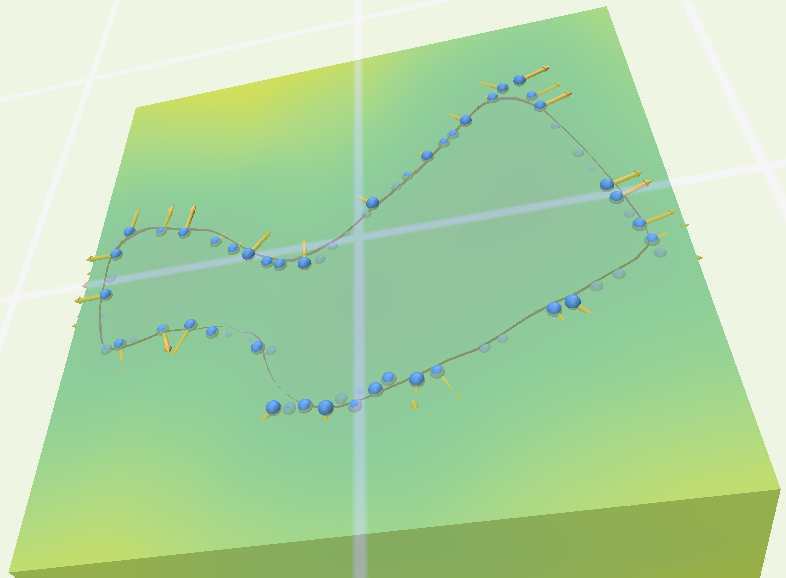
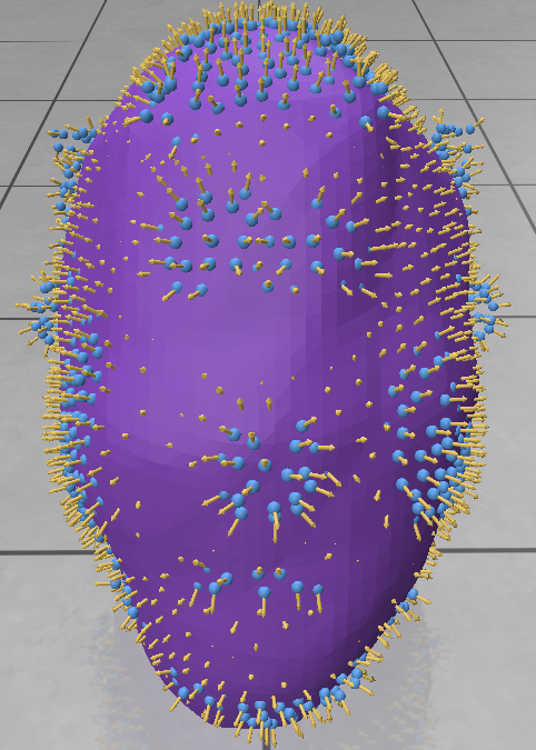
As we can see from the image below, our reconstruction still has a way to go, however, there are still many ideas we still could test: How do the architectures influence the training? Which is the best function to reduce the influence of the adversarial loss terms during training? Are all loss terms really necessary?
Overall this is an interesting project that allow us to explore possible solutions to noisy data in 3D, that it’s still far away from being completely explored.