CLIP is a system designed to determine which image matches which piece of text in a group of images and texts.
1. How it works:
• Embedding Space: Think of this as a special place where both images and text are transformed into numbers.
• Encoders: CLIP has two parts that do this transformation:
– Image Encoder: This part looks at images and converts them into a set of numbers (called embeddings).
– Text Encoder: This part reads text and also converts it into a set of numbers(embeddings).
2. Training Process:
• Batch: Imagine you have a bunch of images and their corresponding texts in a group(batch).
• Real Pairs: Within this group, some images and texts actually match (like an image of a cat and the word ”cat”).
• Fake Pairs: There are many more possible combinations that don’t match (like an image of a cat and the word ”dog”).
3. Cosine Similarity: This is a way to measure how close two sets of numbers (embeddings) are. Higher similarity means they are more alike.
4. CLIP’s Goal: CLIP tries to make the embeddings of matching images and text (real pairs) as close as possible. At the same time, it tries to make the embeddings of non-matching pairs (fake pairs) as different as possible.
5. Optimization:
• Loss Function: This is a mathematical way to measure how good or bad the current matchings are.
• Symmetric Cross-Entropy Loss: CLIP uses a specific type of loss function that looks at the similarities of both real and fake pairs and adjusts the embeddings to improve the matchings.
In essence, CLIP learns to accurately match images and texts by continuously improving how it transforms them into numbers so that correct matches are close together and incorrect ones are far apart.
After learning CLIP, I chose my data set and got to work:
The Describable Textures Dataset (DTD) is an evolving collection of textural images in the wild, annotated with a series of human-centric attributes, inspired by the perceptual properties of textures.
The package contains:
1. Dataset images, train, validation, and test.
2. Ground truth annotations and splits used for evaluation.
3. imdb.mat file, containing a struct holding file names and ground truth labels.
Example images:

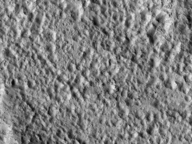

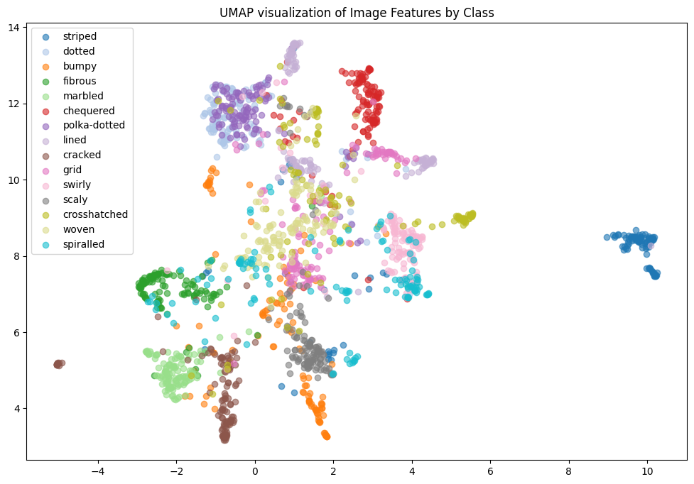
There are 47 texture classes, with 120 images each for a total of 5640 images in this data set. The above shows ‘cobwebbed’, ‘pitted,’ and ‘banded’. I did the t-SNE visualization by class for all the classes but realized this wasn’t very helpful for analysis. It was the same for UMAP. So I decided to sample 15 classes and then visualize:
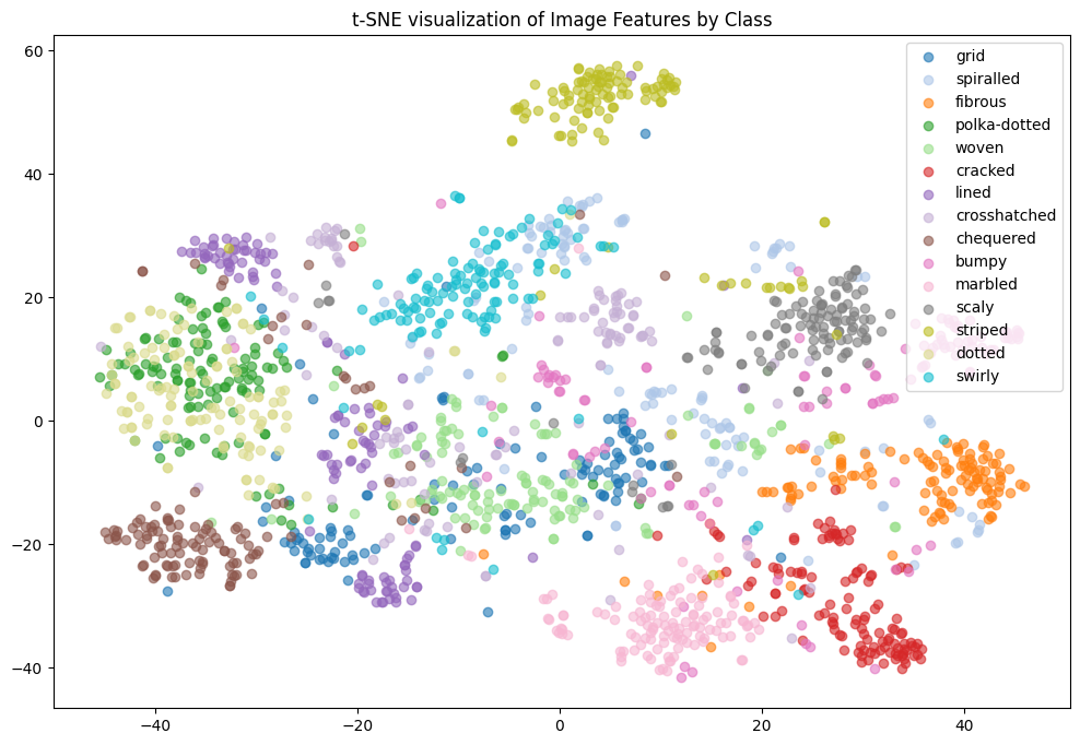
In the t-SNE for 15 classes, we see that ’polka-dotted’ and ’dotted’ are clustered together. This intuitively makes sense. To further our analysis, we computed the subspace angles between the classes. Many pairs of categories have an angle of 0.0, meaning their feature vectors are very close to each other in the feature space. This suggests that these textures are highly similar or share similar feature representations. For instance:
• crosshatched and striped
• dotted and grid
• dotted and polka-dotted
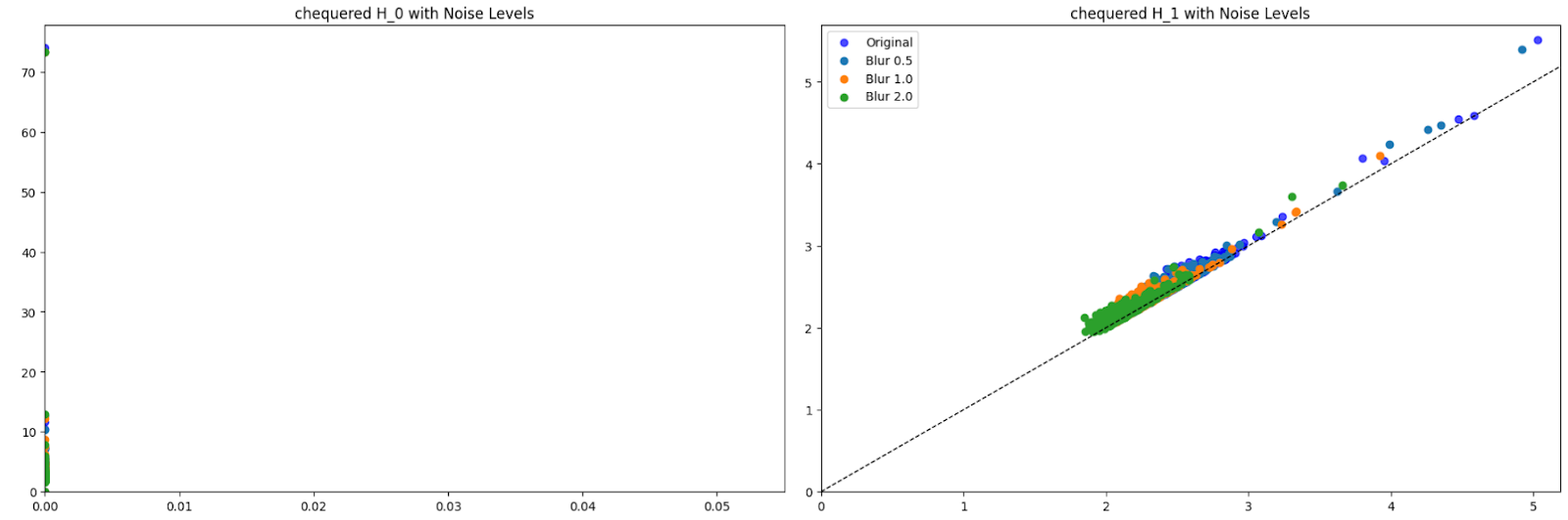
Then came the tda: A persistence diagram summarizes the topological features of a data set across multiple scales. It captures the birth and death of features such as connected components, holes, and voids as the scale of observation changes. In a persistence diagram, each feature is represented as a point in a two-dimensional space, where the x-coordinate corresponds to the “birth” scale and the y-coordinate corresponds to the “death” scale. This visualization helps in understanding the shape and structure of the data, allowing for the identification of significant features that persist across various scales while filtering out noise.
I added 3 levels of noise (0.5, 1.0, 2.0) to the images and then extracted features. I visualized these features on a persistence diagram. Here are some examples of those results. We can see that for H_0 at all noise levels, there is one persistent feature so there is one connected component. The death of this persistent feature varies slightly. H_1 at all noise levels there aren’t any highly persistent features, with most points being around the diagonal. The features in H_1 tend to “clump up together” and die quicker as the noise level goes up.


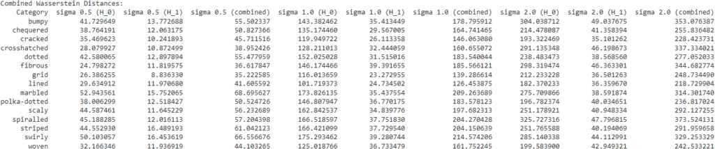
I then computed the distances between the diagrams with no noise and those with noise. Here are some of those results. Unsurprisingly, with greater levels of noise, there is greater distance.
Finally, we wanted to test the robustness of CLIP so we classified images with respect to noise. The goal was to see if the results we saw with respect to the topology of the feature space corresponded to the classification results. These were the classification accuracies:

We hope to discuss our results further!