Month: July 2025

A Derivation of the Force Density Method

Post author By skyler
Post date July 31, 2025

Thanks to Ioannis Mirtsopoulos, Elshadai Tegegn, Diana Avila, Jorge Rico Esteban, and Tinsae Tadesse for invaluable assistance with this article.

A truss is a collection of rigid beams connected together with joints which can rotate, but not slip by each other. Trusses are used throughout engineering, architecture, and other structural design; you’ll see them in railway bridges, supporting ceilings, and forming the foundation for many older roller coasters. When designing trusses, it is often necessary to design for static equilibrium; that is, such that the forces at each joint in the truss sum to zero, and the truss
does not move. One of the most effective ways to accomplish this is by parameterizing our graphs through the ratios between the axial force along each edge and the length of that edge. Our goal for this article is to show that these force-densities parametrize graphs in static equilibrium, subject to certain constraints.

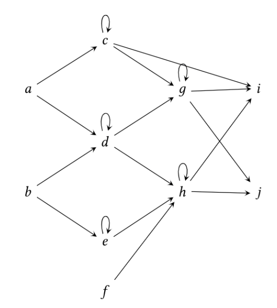
The first constraint we will place upon our system is topological. Recall that a graph is a collection of vertices, together with a collection of edges linking pairs of those vertices. We will fix, once and for all, a graph $G$ to represent the topology of our truss. We will also designate some of the vertices of our graph as fixed vertices and the rest as free vertices. The fixed vertices represent vertices which are attached to some solid medium external to the truss, and so experience normal forces which cancel out any forces which are present from the loading of the truss. In addition to these fixed vertices, to each free vertex we assign a load, which represents the force placed on that point.

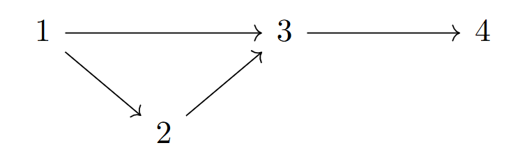
First we introduce the incidence matrix of a (directed)
graph. Recall that a directed graph where the edges have a destinguished ‘first’ vertex; that is, the edges are represented by ordered pairs rather than sets. Given such a graph, the incidence matrix of the graph is the matrix having in the $i,j$-th position a 1 if the $i$-th edge begins with the
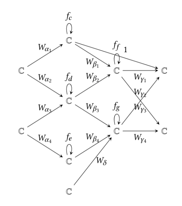
$j$-th vertex, a $-1$ if the $i$-th edge ends with the $j$-th vertex, and a 0 otherwise. We split the entire adjacency matrix $A$ of our graph $G$ into two matrices, $C$ and $C_f$, where $C$ consists of the columns of $A$ which correspond to free vertices, and $C_f$ consists of those columns corresponding to fixed vertices. We will also work with the vectors $p_x$ and $p_y$ of forces, and
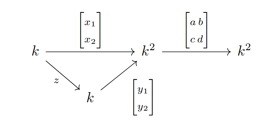
the vectors $x_f$ and $y_f$ of equilibrium points. We wish to construct a map \[F:\mathscr Q \to \mathscr C\]
where $\mathscr Q$ is the space of vectors $q = (q_1, …, q_n)$ of force-length ratios, and $\mathscr C$ is the space of all possible lists of coordinate pairs $(x, y) = (x_1, …, x_n, y_1,
…, y_n)$. It turns out that the map we want is \[F(q) = \left(D^{-1}(p_x – D_fx_f), D^{-1}(p_y – D_fy_f)\right)\]
Where we set $D = C^TQC, D_f = C^TQC_f$, and $Q$ is the diagonal matrix with the $q_i$ along the diagonal. Clearly, this map is a rational map in the $q_i$, and is regular away from where $\det(D) = 0$ (when viewed as a function of $q$).

Derivation

We suppose we have a system with free coordinate vectors $(x, y) = (x_1, …, x_n, y_1, …, y_n)$ and fixed coordinate vectors $(x_f, y_f) = (x_{1f}, …, y_{1f}, …)$ which is
in static equilibrium. First note that we can easily obtain the vectors of coordinate differences $u$ and $v$ (in the $x$ and $y$ directions respectively) using the incidence matrices $C$ and $C_f$.
\[u = Cx + C_fx_f\]
\[v = Cy + C_fy_f\]
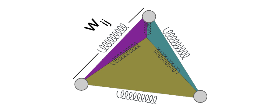
We form the diagonal matrices $U$ and $V$ corresponding to $u$ and $v$, letting $L$ be the matrix with the lengths of the edges down the diagonal and $s$ the vector of axial forces along each edge. We note that if we divide the axial force along each edge by that edge’s length, and then multiply by the length in the $x$ or $y$ direction, we have then calculated the force that edge contributes to each vertex at it’s ends. Multiplying on the left by the transpose of the incedence matrix $C$ then gives the total force on the vertex from all the bars coincident with it, which must then be
equal to the external load applied. This yields the equations
\[C^TUL^{-1}s = p_x,\ \ \ C^TVL^{-1}s = p_y,\]
which hold if and only if the system is in equilibrium. We define $q=L^{-1}s$ to be the vector of force densities, simplifying our equations to
\[C^TUq = p_x,\ \ \ C^TVq = p_y.\]
We note that $Uq = Qu$ and $Vq=Qv$, by the definition of matrix multiplication (each matrix is a diagonal matrix!). Thus we obtain by the definitions of $u$ and $v$
\[p_x = C^TUq = C^TQ(Cx+C_fx_f) = C^TQCx+C^TQC_fx_f, \]
\[p_y = C^TVq = C^TQ(Cy+C_fy_f) = C^TQCy+C^TQC_fy_f.\]
We set, as above, $D = C^TQC$ and $D_f = C^TQC_f$, yielding
\[p_x – D_fx_f= Dx , \]
\[p_y – D_fy_f= Dy ,\]
or as promised
\[D^{-1}(p_x – D_fx_f)=x ,\]
\[D^{-1}(p_y – D_fy_f)=y .\]
Clearly these equations hold if and only if the system is in equilibrium. Since every system (in equilibrium or not) has force densities, this yields an important corallary: Every system which is in equilibrium is of the form $F(q)$ for some choice of force-density ratios $q$, and no system which is not in equilibrium is of such a form.

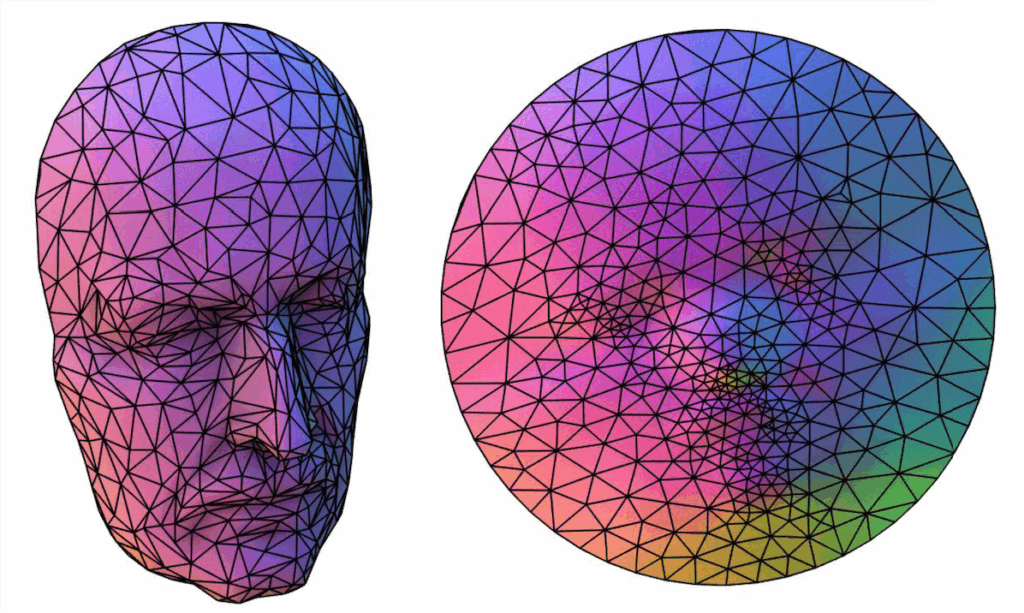
It turns out to be incredibly useful to have this method to parametrize the set of all graphs in static equilibrium. This method is used to calculate the deformation of nets, cloth, and to design load-bearing trusses; it is also used to generate trusses based on particular design parameters. In
a later article we will also describe how one can use FDM to find an explicit representation for the set of possible point configurations which are in static equilibrium.

Post author By skyler
Post date July 31, 2025

Tutorial week

Tutorial Week Day 4: Texture Optimization

Post author By marina.levay
Post date July 29, 2025

Intro

Now that you’ve gotten the grasp of meshes, and created your very first 3D object on Polyscope, what can we do next? On Day 4 of the SGI Tutorial Week, we had speakers Richard Liu and Dale Decatur from the Threedle Lab at UChicago explaining about Texture Optimization.

In animated movies and video games, we are used to observing them with realistic textures. Intuitively, we might imagine that we have this texture as a map applied as a flat “sticker” over it. However, we know from some well-known examples in cartography that it is difficult to create a 2D map of a 3D shape like the Earth without introducing distortions or cuts.

Besides, ideally, we would want to be able to transition from the 2D to the 3D map interchangeably. Framing this 2D map as a function on $\mathbb{R^2}$, we would like it to be bijective.

The process of creating a bijective map from a mesh S in $\mathbb{R^3}$ to a given domain $\Omega$, or $F: \Omega \leftrightarrow S$, is known as mesh parametrization.

UV Unwrapping

Consider a mesh defined by the object as $M = {V, E, F}$, with Vertices, Edges and Faces respectively, where:

\begin{equation*} V \subset R^3 \end{equation*} \begin{align*} E = \{(i, j) \quad &| \text{\quad vertex i is connected to vertex j}\} \\ F = \{(i, j, k) \quad &| \quad \text{vertex i, j , k share a face}\} \end{align*}

For a mesh M, we define the parametrization as a function mapping vertices $V$ to some domain $\Omega$

\begin{equation*} U: V \subset \mathbb{R}^3 \rightarrow \Omega \subset \mathbb{R}^2 \end{equation*}

For every vertex $v_i$ we assign a 2D coordinate $U(v_i) = (u_i, v_i)$ (this is why the method is called UV unwrapping).

This parametrization has a constraint, however. Only disk topology surfaces (those with a 1 boundary loop) surfaces admit a homeomorphism (a continuous and bijective map) to the bounded 2D plane.

As a workaround, we can always introduce a cut.

However, these seams create discontinuities, and in turn, distortions we want to minimize. We can distinguish different kinds of distortions using the Jacobian, the matrix of all first-order partial derivatives of a vector-valued function. Specifically, we look at the singular values of the Jacobian (which in the UV function is defined as a 2×3 matrix per triangle).

\begin{align*} J_f = U\Sigma V^T = U \begin{pmatrix} \sigma_1 & 0 \\ 0 & \sigma_2 \\ 0 & 0 \end{pmatrix} V^T \\ f \text{ is equiareal or area preserving} \Leftrightarrow \sigma_1 \sigma_2 &= 1 \\ f \text{ is equiareal or area preserving} \Leftrightarrow \sigma_1 &= \sigma_2 \\ f \text{ is equiareal or area preserving} \Leftrightarrow \sigma_1 &= \sigma_2 = 1 \end{align*}

We can find the Jacobians of the UV map assignment $U$ using the mesh gradient operator $G \in \mathbb{R}^{3|F|\times V}$

\begin{align*} GU = J \in \mathbb{R}^{3|F|\times V} \end{align*}

The classical approach for optimizing a mesh parametrization is viewing the mesh surface as the graph of a mass-spring system (least squares optimization problem). The mesh vertices are the nodes (with equal mass) with each edge acting as a spring with some stiffness constant.

Two key design choices in setting up this problem are:

Where to put the boundary?
How to set the spring weights (stiffness)?

To compute the parametrization, we minimize the sum of spring potential energies.

\begin{align*} \min_U \sum_{\{i, j\} \in E} w_ij || u_i – u_j||^2 \end{align*}

Where $u_i = (u_i, v_i)$ is the UV coordinate to vertex i. We then aim to solve the ODE:

\begin{align*} \frac{\partial E}{\partial u _i }= \sum_{j \in N_i} 2 \cdot w_{ij} (u_i – u_j) = 0 \end{align*}

Where $N_i$ indexes all neighbors of vertex $i$. We can now fix the boundary vertices and solve each equation for the remaining $u_i$.

A solution by Tutte (1963) and Floater (1997) was computed such that if the boundary is convex and the weights are positive, the solution is guaranteed to be injective. While an injective map has its limitations in terms of transferring the texture back into the 3D shape, it allows us to easily visualize the 2D map of this shape.

Here, we would need to fix or map a boundary to a circle, where all weights are 1.

An alternative to the classical approach is trivial parametrization, where we split the mesh up into its individual triangles in a triangle soup and then flatten each triangle (isometric distortion). We would then translate and scale all triangles to be packed into the unit square.

Translation and uniform scaling does not affect the angles, such that we have no angle distortion. So this tells us that this parametrization approach is conformal.

Still, when packing triangles into the texture image, we might need to rescale them so they fit, meaning the areas are not guaranteed to be the same. We can verify this based on the SDF values:

\begin{align*} \sigma_1\sigma_2 \neq 1 \end{align*}

This won’t be too relevant in the end though because all triangles get scaled by the same factor, so that the area of each triangle is preserved up to some global scaler. As a result, we would still get an even sampling of the surface, which is what we would care about, at least intuitively, for texture mapping.

However, applying a classical algorithm to trivial parametrization is typically a bad solution because it introduces maximal cuts (discontinuities). How can we overcome this issue?

Parametrization with Neural Networks

Assume we have some parametrized function and some target value. With an adaptive learning algorithm, we determine the direction in which to change our parameters so that the function moves closer to our target.

We compute some loss or measure of closeness between our current function evaluation and our target value.We then compute the gradient of this loss with respect to our parameters. Take a small step in that direction. We would repeat this process until we ideally achieved the global minimum.

Similarly, we can use an approach to optimize the mesh texture.

Parametric function = rendering function
Parameters = texture map pixel values (texel = texture pixel)
Target = existing images of the object with the desired colors
Loss = pixel differences between our rendered images and target images.

What happens if we do this? We do achieve a texture map, but each pixel is mostly optimized independently. As a result, the texture ends up more grainy.

Improving Smoothness

What can we do to improve this? Well, we would want to make the function more smooth. For this, we can optimize a new function $\phi(u, v) : \mathbb{R}^2 \rightarrow \mathbb{R}^2$ that maps the texels to RGB color values. By smoothness in $\phi$, we mean that $\phi$ is continuous.

To get the color at any point in the 2D texture map, we just need to query $\phi$ at that UV coordinate!

To encourage smoothness in $\phi$, we can use a 3D coordinate network.

Consider a mapping from a 3D surface to a 2D texture. We can learn a 3D coordinate $\phi$: $\mathbb{R}^3 \rightarrow \mathbb{R}^2$ that maps 3D surface points to RGB colors. $\phi(x, y, z) = (R, G, B)$.

We can then use the inverse map to go from 2D texture coordinates to 3D surface points, then query those points with the coordinate network to get colors, then map those colors back to the 2D texture for easy rendering.

How to compute an inverse map?

We aim to have a mapping from texels to surface poitns, but we already have a mapping from the vertices to the texel plane. The way we can map an arbitrary coordinate to the surface is through barycentric interpolation, a coordinate system relative to a given triangle. In this system, any points has 3 barycentric coordinates.

Post author By marina.levay
Post date July 29, 2025

Tutorial week

Tutorial Week Day 5: Debugging and Robustness

Post author By singhishree
Post date July 23, 2025

On July 11th, Nicholas Sharp, the creator of the amazing Polyscope library, gave the SGI Community an insightful talk on debugging and robustness in geometry processing—insights that would later save several fellows hours of head-scratching and mental gymnastics. The talk was broadly organized into five parts, each corresponding to a paradigm where bugs commonly arise:

Representing Numbers
Representing Meshes
Optimization
Simulation and PDEs
Geometric Machine Learning

Representing Numbers

The algorithms developed for dealing with geometry are primarily built to work with clean and pretty real numbers. However, computers deal with floats, and sometimes they behave ugly. Floats are computers’ approximations of real numbers. Sometimes, it may require an infinite amount of storage to correctly represent a single number of arbitrary precision (unless you can get away with $π=3.14$). Each floating number can either be represented using 32 bits (single precision) or 64 bits (double precision).

Figure 1. An example of the float32 representation

In the floating realm, we have quirks like:

$(x+y)+z \neq x+(y+z)$
$ a>0, b>0$ but $a+b=a$

It is important to note that floating-point arithmetic is not random; it is simply misaligned with real arithmetic. That is, the same operation will consistently yield the same result, even if it deviates from the mathematically expected one. Possible alternatives to floats are integers and binary fraction representations; however, they come with their own obvious limitations.

Who’s your best friend? The NaN! The NaN is a special “floating-point” computers spit out when they’re asked to perform invalid operations like

$\frac{0}{0}\rightarrow $ NaN
$\sqrt{-1} \rightarrow$ NaN (not $i$ haha)

Every operation against a NaN results in… NaN. Hence, one small slip-up in the code can result in the entire algorithm being thrown off its course. Well then… why should I love NaNs? Because a screaming alarm is better than a silent error. If your algorithm is dealing with positive numbers and it computes $\sqrt{-42}$ somewhere, you would probably want to know if you went wrong.

Well, what are some good practices to minimize numerical error in your code?

Don’t use equality for comparison, use thresholds like: $\left| x – x^* \right| < \epsilon$ or $\frac{\left| x – x^* \right|}{\left| x^* \right|} < \epsilon$
Avoid transcendental functions wherever possible. A really cool example of this is to avoid $\theta = \arccos \left( \frac{ \mathbf{u} \cdot \mathbf{v} }{ \left| \mathbf{u} \right| \left| \mathbf{v} \right| } \right)$ and use $\cot \theta = \frac{ \cos \theta }{ \sin \theta } = \frac{ \mathbf{u} \cdot \mathbf{v} }{ \left| \mathbf{u} \times \mathbf{v} \right| }$ instead.
Clamp inputs to safe bounds, e.g. $\sqrt{x} \rightarrow \sqrt{max(x, 0)}$. (Note that while this keeps your code running smoothly, it might convert NaNs into silent errors!)
Perturb inputs to singular functions to ensure numerical stability, e.g. $\frac{1}{\left| x \right|} \to \frac{1}{\left| x \right| + \epsilon}$

Some easy solutions include:

Using a rational arithmetic system, as mentioned before. Caveats include: 1) no transcendental operations 2) some numbers might require very large integers to represent them, leading to performance issues, in terms of memory and/or speed.
Use robust predicates for specific functional implementations, the design of which is aware of the common floating-point problems

Representing Surface Meshes

Sometimes, the issue lies not with the algorithm but with the mesh itself. However, we still need to ensure that our algorithm works seamlessly on all meshes. Common problems (and solutions) include:

Unreferenced vertices and repeated vertices: throw them out
A mixture of quad and triangular meshes: subdivide, retriangulate, or delete
Degenerate faces and spurious topology: either repair these corner cases or adjust the algorithm to handle these situations
Non-manifold and non-orientable meshes: split the mesh into multiple manifolds or orientable patches
Foldover faces, poorly tessellated meshes, and disconnected components: use remeshing algorithms like Instant Meshes or use Generalized Winding Numbers instead of meshes

Optimization

Several geometry processing algorithms involve optimization of an objective function. Generally speaking, linear and sparse linear solvers are well-behaved, whereas more advanced methods like gradient descent or non-linear solvers may fail. A few good practices include:

Performing sanity checks at each stage of your code, e.g. before applying an algorithm that expects SPD matrices, check if the matrix you’re passing is actually SPD
When working with gradient-descent-like solvers, check if the gradient magnitudes are too large; that may cause instability for convergence

Simulations and PDEs

Generally, input meshes and algorithms are co-designed for engineering and scientific computing applications, so there aren’t too many problems with their simulations. However, visual computing algorithms need to be robust to arbitrary inputs, as they are typically just one component of a larger pipeline. Algorithms often fail when presented with “bad” meshes, even if it is perfect in terms of connectivity (like being a manifold, being oriented, etc.). Well then, what qualifies as a bad mesh? Meshes with skinny or obtuse triangles are particularly problematic. The solution is to remesh them using more equilateral triangles

Figure 2. (Left) An example of a “bad” mesh with skinny triangles. (Middle) A high-fidelity re-mesh that might be super-expensive to process. (Right) A low-fidelity re-mesh that trades fidelity for efficiency.

Geometric Machine Learning

Most geometric machine learning stands very directly atop geometry processing; hence, it’s important to get it right. The most common problems encountered in geometric machine learning are not so different from those encountered in standard machine learning. These problems include:

Array shape errors: You can use the Python aargh library to monitor and validate tensor shapes
NaNs and infs: Maybe your learning rate is too big? Maybe you’re passing bad inputs into singular functions? Use torch.autograd.set_detect_anomaly(mode, check_nan=True) to track these problematic numbers at inception.
“My trained model works on shape A, but not shape B.”: Is your normalization, orientation, and resolution consistent?

It is a good idea to overfit your ML model on a single shape and ensure that it works on simple objects like cubes and spheres before moving on to more complex examples.

And above all, the golden rule when your algorithm fails:
Visualize everything.

Post author By singhishree
Post date July 23, 2025

Talks

Week 2: Guest Lecture

Post author By mhellinger
Post date July 21, 2025

On Wednesday, July 9th, SGI fellows were treated to a one hour presentation by guest lecturer Aaron Hertzmann, Principal Scientist at Adobe Research in San Francisco, CA. Aaron was introduced by SGI fellow Amber Bajaj, who among other accomplishments, noted that Aaron was recently recognized by the Association for Computing Machinery (ACM)’s SIGGRAPH professional society “for outstanding achievement in computer graphics and interactive techniques” and correspondingly awarded the Computer Graphics Achievement Award. The title of the talk was “Toward a Theory of Perspective: Perception in Pictures” and began on a personal note, with Aaron conveying how he was often critical of his own art differing from the corresponding photo he would take of the scene he was illustrating.

From that anecdotal example, Aaron expanded his talk to cover topics of human perception, vision, theory of perspective, and much more, weaving it all together to paint a compelling picture of what factors contribute to what we, as humans, perceive as more accurate representations of our three dimensional reality on a two dimensional medium. He made a compelling point that, while single point perspective is typically how cameras capture scenes and that single point linear perspective is a common tenant of formal art classes, multi-point perspective more faithfully represents how we remember our experiences. In a world of electronics, digital imagery, and automation, it was striking how the lecturer made it clear that artists are still able to convey an image more faithful to the experience than digital cameras and rendered three dimensional imagery can capture.

Key points from Aaron’s talk:

Only 3% of classical paintings strictly follow linear perspective
A multi-perspective theory more faithfully captures our experience
MaDCoW (Zhang et al., CVPR 2025) is a warping algorithm that works for a variety of input scenes
99.9% of vision is peripheral, which leads to inattention blindness (object lying outside the focus of our fovea)
We don’t store a consistent single 3-D representation in our head… it is fragmentary across fixations
There are systematic differences between drawings, photographs, and experiments

Finally, the lecture came full circle with Aaron returning to the art piece he presented at the start and noting seven trends he’s identified from his own work that merit further research: good agreement with linear perspective in many case; distant object size, nearby object size; fit to canvas shape; reduced / eliminated foreshortening; removed objects and simplified shapes; multiperspective for complex composition. Overall the lecture was thought provoking and motivational for the fellows currently engrossed in the 2025 Summer Geometry Initiative.

Post author By mhellinger
Post date July 21, 2025

Research

Hidden Quivers: Supporting the Manifold Hypothesis

Post author By stephanie.p.atherton
Post date July 21, 2025

Quivers are a tool that are known to help us simplify problems in math. In particular, representations of quivers contribute to geometric perspectives in representation theory: the theory of reducing complex algebraic structures to simpler ones. Lesser known, neural networks can also be represented using quiver representation theory.

Fundamentally, a quiver is just a directed graph.

Intrinsic definitions to consider include:

A source vertex of a quiver has no edges directed towards it
A sink vertex has no edges directed away from it
A loop in a quiver is an oriented edge such that the start vertex is the same as the end vertex

A fancy type of quiver known as an Auslander-Reiten quiver, courtesy of the author. But remember!, a quiver is simply a directed graph.

Just like an MLP, a network quiver $Q$ is arranged by input, output, and hidden layers in between. Likewise, they also have input vertices (a subset of source vertices), bias vertices (the source vertices that are not input vertices), and output vertices (sinks of $Q$). All remaining vertices are hidden vertices. The hidden quiver $\tilde{Q}$ consists of all hidden vertices $\tilde{V}$ of $Q$ and all oriented edges $\tilde{E}$ between $\tilde{V}$ of $Q$ that are not loops.

Def: A network quiver $Q$ is a quiver arranged by layers such that:

There are no loops on source (input and bias) nor sink vertices.
There exists exactly one loop on each hidden vertex

For any quiver $Q$, we can also define its representation $\mathcal{Q}$, in which we assign a vector space to each vertex of $Q$ and regard our directed edges of $Q$ as $k$-linear maps. In a thin representation, each $k$-linear map is simply a $1\times1$ matrix.

A quiver with 4 vertices, courtesy of the author.

A *representation* of the quiver directly above, courtesy of the author.

Defining a neural network $(W, f)$ over a network quiver $Q$, where $W$ is a specific thin representation and $f = (f_v)_{v \in V}$ are activation functions, allows much of the language and ideas of quiver representation theory to carry over to neural networks .

When a neural network like an MLP does its forward pass, it gives rise to a pointwise activation function $f$, defined here as a one variable non-linear function $f: \mathbb{C} \to \mathbb{C}$ differentiable except in a set of measure zero. We assign these activation functions to loops of $Q$.

Further, for a neural network $(W, f)$ over $Q$, we have a network function

$$ \Psi(W, f): \mathbb{C}^d \to \mathbb{C}^k $$

where the coordinates of $\Psi(W, f)(x)$ are the score of the neural net as the activation outputs of the output vertices of $(W, f)$ with respect to an input data vector $x \in \mathbb{C}^d$.

The manifold hypothesis critical to deep learning proposes that high-dimensional data actually lies in a low-dimensional, latent manifold within the input space. We can map the input space to the geometric moduli space of neural networks $_d\mathcal{M}_k(\tilde{Q})$ so that our latent manifold is also translated to the moduli space. While $_d\mathcal{M}_k(\tilde{Q})$ depends on the combinatorial structure of the neural network, activation and weight architectures of the neural network determine how data is distributed inside the moduli space.

The mobius strip is a well-known geometric manifold.

We will approach the manifold hypothesis via framed quiver representations. A choice of a thin representation $\tilde{\mathcal{Q}}$ of the hidden quiver $\tilde{Q}$ and a map $h$ from the hidden representation $\tilde{\mathcal{Q}}$ to hidden vertices determine a pair $(\tilde{\mathcal{Q}}, h)$, where $h = \{h_v\}{v \in \tilde{V}}$. The pair $(\tilde{\mathcal{Q}}, h)$ is used to denote our framed quiver representation.

Def: A double-framed thin quiver representation is a triple $(l, \tilde{\mathcal{Q}}, h)$ where:

$\tilde{\mathcal{Q}}$ is a thin representation of the hidden quiver $\tilde{Q}$
$(\tilde{\mathcal{Q}}, h)$ is framed representation of $\tilde{Q}$
$(\tilde{\mathcal{Q}}, l)$ is a co-framed representation of $\tilde{Q}$ (the dual of a framed representation)

Denote by $_d\mathcal{R}_k(\tilde{\mathcal{Q}})$ the space of all double-framed thin quiver representations. We will use stable double-framed thin quiver representations in our construction of moduli space.

Def: A double-framed thin quiver representation $\texttt{W}_k^f = (l, \tilde{\mathcal{Q}}, h)$ is stable if :

The only sub-representation of $\tilde{\mathcal{Q}}$ contained in the kernel of $h$ is the zero sub-representation
The only sub-representation of $\tilde{\mathcal{Q}}$ contained in the image of $l$ is $\tilde{\mathcal{Q}}$

Def: We present the moduli space of double-framed thin quiver representations as

$$ _d\mathcal{M}_k(\tilde{Q}):=\{[V]: _d\mathcal{R}_k(\tilde{\mathcal{Q}}) \space \text{is stable} \}. $$

The moduli space depends on the hidden quiver as well as the chosen vector spaces. Returning to neural networks $(W, f)$, and given an input data vector $x \in \mathbb{C}^d$, we can define a map

$$ \varphi(W, f): \mathbb{C}^d \to _d\mathcal{R}_k(\tilde{\mathcal{Q}})\\x \mapsto \texttt{W}_k^f. $$

This map takes values in the moduli space, the points of which parametrize isomorphism classes of stable double-framed thin quiver representations. Thus we have

$$ \varphi(W, f): \mathbb{C}^d \to _d\mathcal{M}_k(\tilde{Q}).
$$

As promised, we have mapped our input space containing our latent manifold to the moduli space $_d\mathcal{M}_k(\tilde{Q})$ of neural networks, mathematically validating the manifold hypothesis.

Independent of the architecture, activation function, data, or task, any decision of any neural network passes through the moduli (as well as representation) space. With our latent manifold translated into the moduli space, we have an algebro-geometric way to continue to study the dynamics of neural network training.

Looking through the unsuspecting the lens of quiver representation theory has the potential to provide new insights in deep learning, where network quivers appear as a combinatorial tool for understanding neural networks and their moduli spaces. More concretely:

Continuity and differentiability of the network function $\Psi(W, f)$ and map $\varphi(W, f)$ should allow us to apply further algebro-geometric tools to the study of neural networks, including to our constructed moduli space $_d\mathcal{M}_k(\tilde{Q})$.
Hidden quivers can aid us in comprehending optimization hyperparameters in deep learning. We may be able to transfer gradient descent optimization to the setting of the moduli space.
Studying training within moduli spaces can lead to the development of new convergence theorems to guide deep learning.
The dimension of $_d\mathcal{M}_k(\tilde{Q})$ could be used to quantify the capacity of neural networks.

The manifold hypothesis has played a ubiquitous role throughout deep learning since originally posed, and formalizing its existence via the moduli of quiver representations can help us to understand and potentially improve upon the effectiveness of neural networks and their latent spaces.

Notes and Acknowledgements. Content for this post was largely borrowed from and inspired by The Representation Theory of Neural Networks, smoothing over many details more rigorously presented in the original paper. We thank the 2025 SGI organizers and sponsors for supporting the author’s first deep learning-related research experience via the “Topology Control” project as well as mentors and other research fellows involved for their diverse expertise and patience.

Author

stephanie.p.atherton

Post author By stephanie.p.atherton
Post date July 21, 2025
Tags Deep Learning, Geometry