Picture your triangle mesh as that poor, crumpled T-shirt you just pulled out of the dryer. It’s full of sharp folds, uneven patches, and you wouldn’t be caught dead wearing it in public—or running a physics simulation! In geometry processing, these “wrinkles” manifest as skinny triangles, janky angles, and noisy curvature that spoil rendering, break solvers, or just look… ugly. Sometimes, we might want to fix these problems using something geometry nerds call surface fairing.
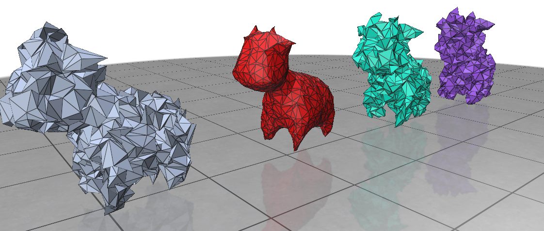
Figure 1. (Left) Clean mesh, (Right) Mesh damaged by adding Gaussian noise to each vertex (Middle) Result after applying surface fairing to the damaged mesh.
In essence, surface fairing is an algorithm one uses to smoothen their mesh. Surface fairing can be solved using energy minimization. We define an “energy” that measures how wrinkly our mesh is, then use optimization algorithms to slightly nudge each vertex so that the total energy drops.
Spring Energy Think of each mesh edge (i,j) as a spring with rest length 0. If a spring is too long, it costs energy. Formally: Emem = ½ Σ(i,j)∈E wij‖xi − xj‖² with weights wij uniform or derived from entries of the discrete Laplacian matrix (using cotangents of opposite angles). We’ll call this term the Membrane Term
Bending Energy Sometimes, we might want to additionally smooth the mesh even if it looks less wrinkly. In this case, we penalize the curvature of the mesh, i.e., the rate at which normals change at the vertices: Ebend = ½ Σi Ai‖Δxi‖² where Δxi is the discrete Laplacian at vertex i and Ai is its “vertex area”. For the uninitiated, the idea of a vertex having an area might seem a little weird. But it represents how much area a vertex controls and is often calculated as one-third of the summed areas of triangles incident to vertex i. We’ll call this energy term the Laplacian Term.
Angle Energy As Nicholas has warned the fellows, sometimes, having long skinny triangles can cause numerical instability. So we might like our triangles to be more equilateral. We can additionally punish deviations from 60° for each triangle, by adding another energy term: Eangle = Σk=1..3(θk−60°)². We’ll call this the Angle Term.
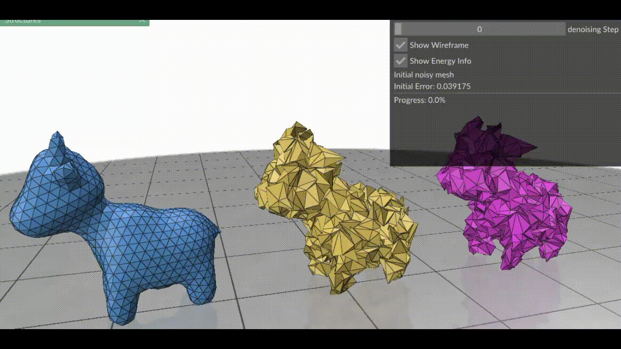
Figure 2. (Left) Damaged mesh. (In order) Surface fairing using only 1) Spring Energy 2) Bending Energy 3) Angle Energy. Notice how the last two energy minimizations fail to smooth the mesh properly alone.
Note that in most cases using angle energy and bending energy terms are optional, but using the spring energy term is important! (however, you may encounter a few special cases where you can make do without the spring energy?? i’m not too sure, don’t take my word for it). Once we have computed these energies, we weight them appropriately with scaling factors and sum them up. The next step is to minimize them. I love Machine Learning and hate numerical solvers; and so, it brings me immense joy to inform you that since the problem is non-convex, we can should use gradient descent! At each vertex, compute the gradient ∇xE and take a tiny step towards the minima: \(x_{i} \leftarrow x_i – \lambda \cdot (\nabla_{x} E)_{i}\)
Now, have a look at our final surface fairing algorithm in its fullest glory. Isn’t it beautiful? Maybe you and I are nerds after all 🙂
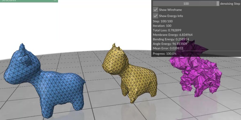
Figure 1. (Left) Clean mesh, (Right) Damaged mesh (Middle) Resulting mesh after each step of gradient descent on the three energy terms combined. Note how the triangles in this case are more equilateral than the red mesh in Figure 2, because we’ve combined all energy terms.
So, the next time your mesh looks like you’ve tossed a paper airplane into a blender, remember: with a bit of math and a few iterations, you can make it runway-ready; and your mesh-processing algorithm might just thank you for sparing its life. You can find the code for the blog at github.com/ShreeSinghi/sgi_mesh_fairing_blog.
Happy geometry processing!
References
Desbrun, M., Meyer, M., Schröder, P., & Barr, A. H. (1999). Implicit fairing of irregular meshes using diffusion and curvature flow.
Pinkall, U., & Polthier, K. (1993). Computing discrete minimal surfaces and their conjugates.
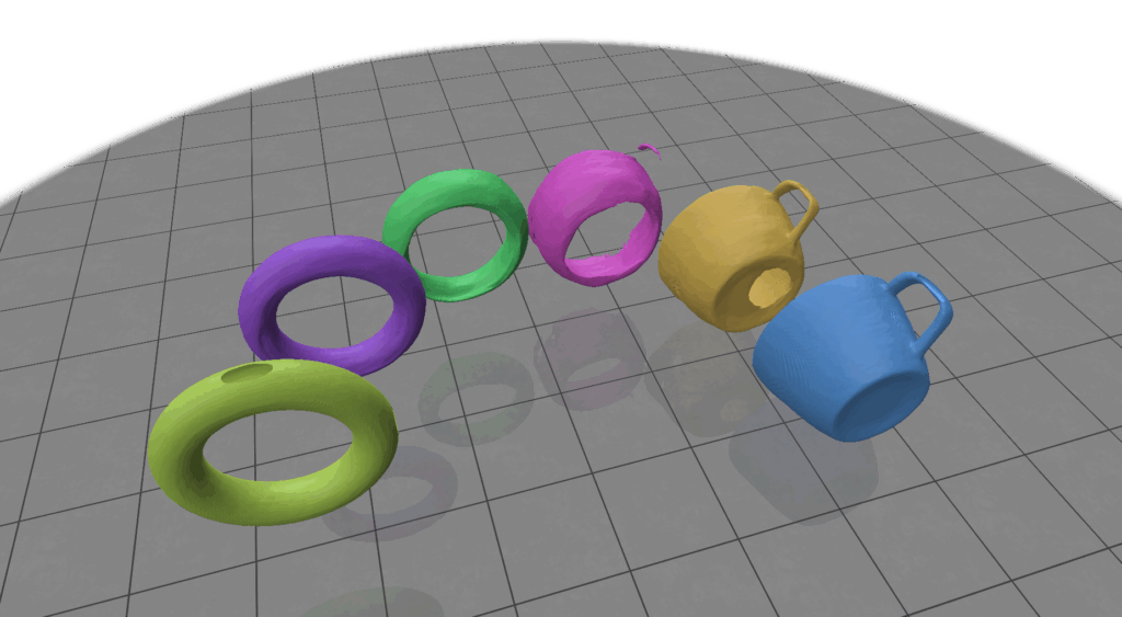
In the Topology Control project mentored by Professor Paul Kry and project assistants Daria Nogina and Yuanyuan Tao, we sought to explore preserving topological invariants of meshes within the framework of DeepSDFs. Deep Signed Distance Functions are a neural implicit representation used for shapes in geometry processing, but they don’t come with the promise of respecting topology. After finishing our ML pipeline, we explored various topology-preserving techniques through our simple, initial case of deforming a “donut” (torus) into a mug.
DeepSDFs
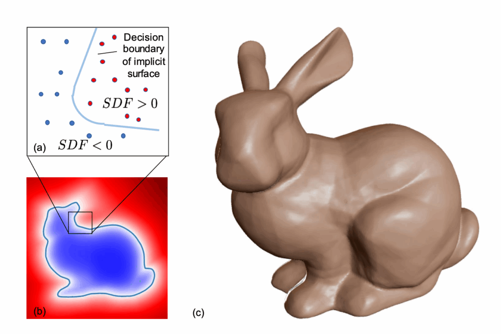
Signed Distance Field (SDF) representation of a 3D bunny. The network predicts the signed distance from each spatial point to the surface. Source: (Park et al., 2019).
Signed Distance Functions (SDFs) return the shortest distance from any point in 3D space to the surface of an object. Their sign indicates spatial relation: negative if the point lies inside, positive if outside. The surface itself is defined implicitly as the zero-level set: the locus where \(\text{SDF}(x) = 0 \).
In 2019, Park et al. introduced DeepSDF, the first method to learn a continuous SDF directly using a deep neural network (Park et al., 2019). Given a shape-specific latent code \( z \in \mathbb{R}^d \) and a 3D point \( x \in \mathbb{R}^3 \), the network learns a continuous mapping:
$$ f_\theta(z_i, x) \approx \text{SDF}^i(x), $$
where \( f_\theta \) takes a latent code \( z_i \) and a 3D query point \( x \) and returns an approximate signed distance.
The training set is defined as:
$$ X := {(x, s) : \text{SDF}(x) = s}. $$
Training minimizes the clamped L1 loss between predicted and true distances:
Clamping focuses the loss near the surface, where accuracy matters most. The parameter \( \delta \) sets the active range.
This is trained on a dataset of 3D point samples and corresponding signed distances. Each shape in the training set is assigned a unique latent vector \( z_i \), allowing the model to generalize across multiple shapes.
Once trained, the network defines an implicit surface through its decision boundary, precisely where \( f_\theta(z, x) = 0 \). This continuous representation allows smooth shape interpolation, high-resolution reconstruction, and editing directly in latent space.
Training Field Notes
We sampled training data from two meshes, torus.obj and mug.obj using a mix of blue-noise points near the surface and uniform samples within a unit cube. All shapes were volume-normalized to ensure consistent interpolation.
DeepSDF is designed to intentionally overfit. Validation is typically skipped. Effective training depends on a few factors: point sample density, network size, shape complexity, and sufficient epochs.
After training, the implicit surface can be extracted using Marching Cubes or Marching Tetrahedra to obtain a polygonal mesh from the zero-level set.
Training Parameters
SDF Delta
1.0
Latent Mean
0.0
Latent SD
0.01
Loss Function
Clamped L1
Optimizer
Adam
Network Learning Rate
0.001
Latent Learning Rate
0.01
Batch Size
2
Epochs
5000
Max Points per Shape
3000
Network Architecture
Latent Dimension
16
Hidden Layer Size
124
Number of Layers
8
Input Coordinate Dim
3
Dropout
0.0
Point Cloud Sampling
Radius
0.02
Sigma
0.02
Mu
0.0
Number of Gaussians
10
Uniform Samples
5000
For higher shape complexity, increasing the latent dimension or training duration improves reconstruction fidelity.
Latent Space Interpolation
One compelling application is interpolation in latent space. By linearly blending between two shape codes \( z_a \) and \( z_b \), we generate new shapes along the path
$$ z(t) = (1 – t) \cdot z_a + t \cdot z_b,\quad t \in [0,1]. $$
Latent space interpolation between mug and torus.
While DeepSDF enables smooth morphing between shapes, it exposes a core limitation: a lack of topological consistency. Even when the source and target shapes share the same number of genus, interpolated shapes can exhibit unintended holes, handles, or disconnected components. These are not artifacts, they reveal that the model has no built-in notion of topology.
However, this limitation also opens the door for deeper exploration. If neural fields like DeepSDF lack an inherent understanding of topology, how can we guide them toward preserving it? In the next post, we explore a fundamental topological property—genus—and how maintaining it during shape transitions could lead us toward more structurally meaningful interpolations.
I kicked off this project with my advisor, Yu Wang, over Zoom the weekend before our official start, checked in mid-week to ask questions and provide a progress report, and wrapped up the week with a final Zoom review—each meeting improving my understanding of the fundamental problem and how to improve my approach in Python. I’m excited to share these quasi-harmonic ideas of how a blend of PDE insight and mesh-based propagation can yield both speed and exactness in geodesic computation.
Finding the shortest path on a curved surface—called the geodesic distance—is deceptively challenging. Exact methods track how a wavefront would travel across every triangle of the mesh, which is accurate but can be painfully slow on complex shapes. The Heat Method offers a clever shortcut: imagine dropping a bit of heat at your source point, let it diffuse for a moment, then “read” the resulting temperature field to infer distances. By solving two linear systems—one for the heat spread and one to recover a distance‐like potential—you get a fast, global approximation. It runs in near-linear time and parallelizes beautifully, but it can smooth over sharp creases and slightly misestimate in highly curved regions.
To sharpen accuracy where it matters, I adopted a hybrid strategy. First, detect “barrier” edges—those sharp creases where two faces meet at a steep dihedral angle—and temporarily slice the mesh along them. Then apply the Heat Method independently on each nearly‐flat patch, pinning the values along the cut edges to their true geodesic distances. Finally, stitch everything back together by running a precise propagation step only along those barrier edges. The result is a distance field that retains the Heat Method’s speed and scalability on smooth regions, yet achieves exactness along critical creases. It’s remarkable how something as seemingly simple as measuring distance on a surface can lead into rich territory—mixing partial-differential equations, sparse linear algebra, and discrete geometry in pursuit of both efficiency and precision.
Differential geometry makes heavy use of calculus in order to study geometric objects such as smooth manifolds. Just as differential geometry builds upon calculus and other fundamentals, the notion of differential forms extend the approaches of differential geometry and calculus, even allowing us to study the larger class of surfaces that are not necessarily smooth. We will motivate from calculus a brief brush with differential forms and their geometric potential.
Review of Vector Fields
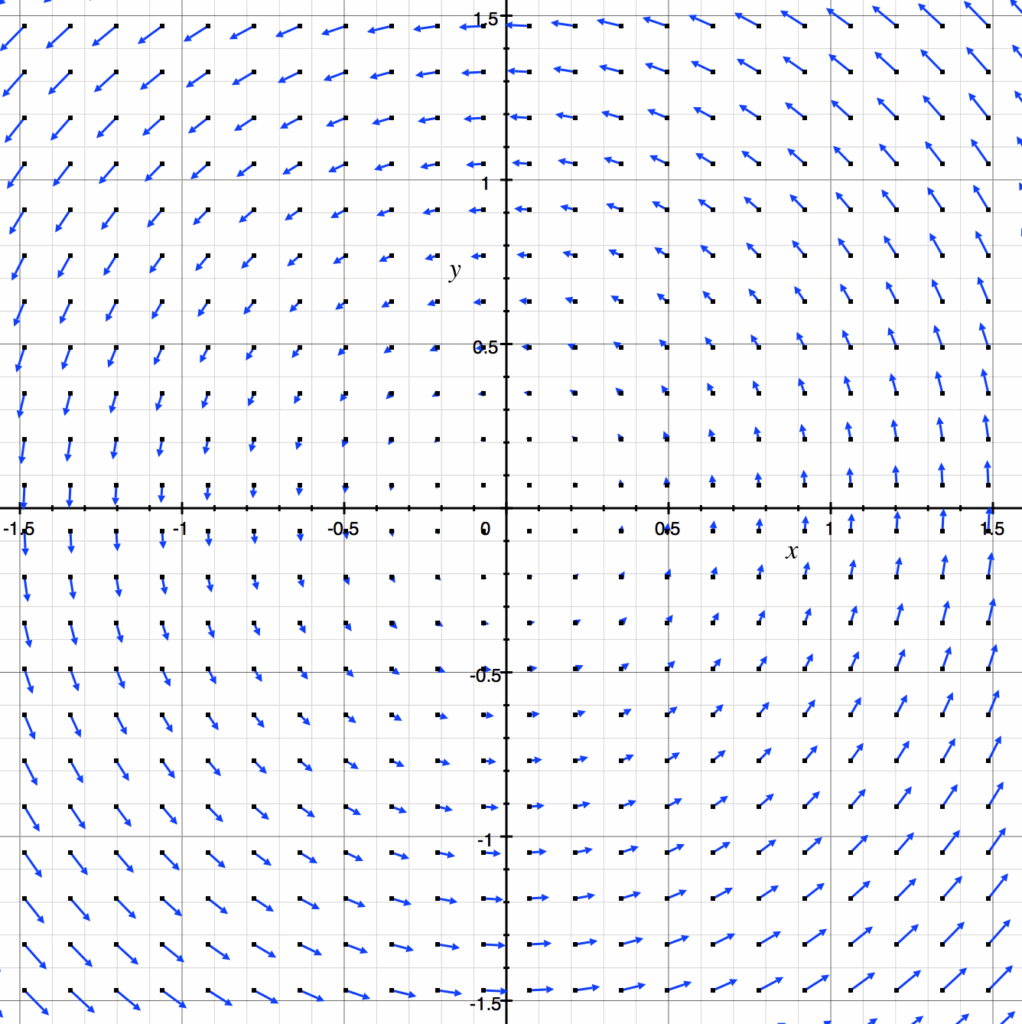
Recall a vector field is a special case of a multivariable vector-valued function (taking in a scalar or a vector and outputting a set of multidimensional vectors). Often they are defined in \(\mathbb{R}^2\) or \(\mathbb{R}^3\), but can also be defined more generally on smooth manifolds.
In three dimensional space, a vector field is a function \(V\) that assigns to each point \((x, y, z)\) a three dimensional vector given by \(V(x, y, z)\). Consider our identity function
$$ V(x, y, z) = \begin{bmatrix}x\\y\\z \end{bmatrix}, $$
where for each point \((x, y, z)\) we associate a vector with those same coordinates. Generalizing, for any vector function \(V(x, y, z)\), we visualize its vector field by placing the tail of the corresponding vector \(V(x_0, y_0, z_0)\) at its point \((x_0, y_0, z_0)\) in the domain of \(V(x, y, z)\).
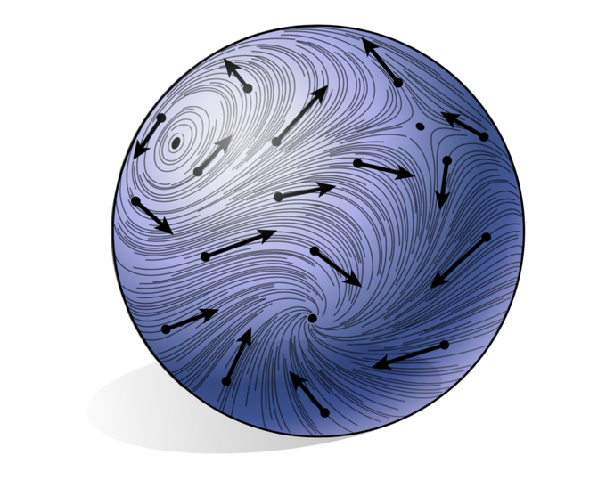
Here we consider fluid particles (displayed as blue dots) as points, each with its own magnitude, direction, and velocity that correspond to overall fluid flow. Then to each point in our sample of particles we can assign a vector with speed of velocity as its length. Each arrow not only represents the velocity of the individual particle it is attached to, but also takes into account how the neighborhood of particles around it move.
Vector fields can be transformed into scalar fields via \(\nabla\) taken as a vector differentiable operator known as the gradient operator.
Our gradient points in the direction of steepest ascent of a scalar function \(f(x_1, x_2, x_3, . . . x_n)\), indicating the direction of greatest change of \(f\). A vector field \(V\) over an open set \(S\) is agradient fieldif there exists a differentiable real-valued function (the scalar field) \(f\) on \(S\). Then
is a special type of vector field \(V\) defined as the gradient of a scalar function, where each \( v \in V\) is the gradient of \(f\) at that point.
The Divergence and Curl Operators
Now that we have reviewed vector fields, recall that we can also perform operations like divergence and curl over them. When fluid flows over time, some regions of fluid will become less dense with particles as they flow away (negative divergence). Meanwhile, particles tending towards each other will cause the fluid in that region to be more dense (positive divergence).
Luckily, we have our handy divergence operator to take in the vector-valued function of our vector field and output a scalar-valued function measuring the change in density of the fluid around each point. Given a vector field \(V\), we can think of divergence
as a variation of the derivative that generalizes to vector fields \(V\) of any dimension. Another “trick” to thinking about the divergence formula is as the trace of the Jacobian matrix of the vector field.
In differential geometry, one can also define divergence on a Riemannian manifold \((M, g)\), a smooth manifold \(M\) endowed with the Riemannian metric \(g\) as a choice of inner product for each tangent space of \(M\).
The Riemannian metric allows us to take the inner product of the two vectors tangent to the sphere.
Whereas divergence describes changes in density, curl measures the “rotation”, or angular momentum, of the vector field \(V\). Likewise, the curl operator takes in a vector-valued function and outputs a function that describes the flow of rotation given by the vector field at each point.
Here, all the points go in circles in the counterclockwise direction, which we define by \(V(x, y) = \begin{bmatrix} -y \\ x \end{bmatrix} = -y\hat{i} + x\hat{j}\).
we can look at the change of a point \((x_0, y_0)\) by looking at the change in \(v_1\) as \(y\) changes and \(v_2\) as \(x\) changes. We calculate
$$2\text{d curl} \space V = \nabla \times V = \frac{\partial v_2}{\partial x}(x_0, y_0) \space – \frac{\partial v_1}{y}(x_0, y_0),$$
with a positive evaluation indicating counterclockwise rotation around \((x_0, y_0)\) and a negative evaluation indicating clockwise.
Approach by Differential Forms
Vector calculus can also be viewed more generally and geometrically via the theory of differential forms.
While curl is typically only defined in two and three dimensions, it can be generalized in the context of differential forms. The calculus of differential \(k\)-forms offers a unified approach to define integrands over curves, surfaces, and higher-dimensional manifolds. Differential 1-forms of expression form
$$\omega = f(x)dx$$
are defined on an open interval \( U \subseteq \mathbb{R^n}\) with \(f: U \to \mathbb{R}\) a smooth function. We can have 1-forms
$$\omega = f(x, y)dx + g(x, y)dy$$
defined on an open subset \( U \subseteq \mathbb{R^2}\) ,
$$\omega = f(x, y, z)dx + g(x, y, z)dy + h(x, y, z)dz $$
defined on an open subset \( U \subseteq \mathbb{R^3}\), and so on for any positive integer \(n\).
Correspondence Theorem: Given a 1-form \(\omega = f_1dx_1 + f_2dx_2 + . . . f_ndx_n\), we can define an associated vector field with component functions \((f_1, f_2, . . . f_n)\). Conversely, given a smooth vector field \(V = (f_1, f_2, . . . f_n)\), we can define an associated 1-form \(\omega = f_1dx_1 + f_2dx_2 + . . . f_ndx_n\).
Via the exterior derivative and an extension of the correspondence between 1-forms and vector fields to arbitrary \(k\)-forms, we can generalize the well-known operators of vector calculus.
The exterior derivative \(d\omega\) of a \(k\)-form is simply a \(k + 1\)-form. We provide an example of its use in defining curl:
Let \(\omega = f(x, y, z)dx + g(x, y, z)dy + h(x, y, z)dz\) be a 1-form on \( U \subseteq \mathbb{R}^3\) with its associated vector field \(V = (f, g, h)\). Its exterior derivative \(d\omega\) is the 2-form
as the vector field associated to the 2-form \(d\omega\). Attempt to see how this definition of curl agrees with the traditional version, but can be applied in higher dimensions.
The natural pairing between vector fields and 1-forms allows for the modern approach of \(k\)-forms for multivariable calculus and has also heavily influenced the area of geometric measure theory(GMT), where we define currents as functionals on the space of \(k\)-forms. Via currents, we have the impressive result that a surface can be uniquely defined by the result of integrating differential forms over it. Further, the differential forms fundamental to GMT open up our toolbox to studying geometry that is not necessarily smooth!
Acknowledgements. We thank Professor Chien, Erick Jiminez Berumen, and Matheus Araujo for exposing us to new math, questions, and insights, as well as for their mentorship and dedication throughout the “Developing a Medial Axis for Measures” project. We also acknowledge Professor Solomon for suggesting edits incorporated into this post, as well as for his organization of the wonderful summer program in the first place!