SGI Fellows: Lydia Madamopoulou, Nhu Tran, Renan Bomtempo and Tiago Trindade
Mentor. Yusuf Sahillioglu
SGI Volunteer. Eric Chen
Introduction
In the world of 3D modeling and computational geometry, tackling geometrically complex shapes is a significant challenge. A common and powerful strategy to manage this complexity is to use a “divide-and-conquer” approach, which partitions a complex object into a set of simpler, more manageable sub-shapes. This process, known as shape decomposition, is a classical problem, with convex decomposition and star-shaped decomposition being of particular interest.
The core idea is that many advanced algorithms for tasks like creating volumetric maps or parameterizing a shape are difficult or unreliable on arbitrary models, but work perfectly on simpler shapes like cubes, balls, or star-shaped regions.
The paper by Hinderink et al. (2024) demonstrates this perfectly. It presents a method to create a guaranteed one-to-one (bijective) map between two complex 3D shapes. They achieve this by first decomposing the target shape into a collection of non-overlapping star-shaped pieces. By breaking the hard problem down into a set of simpler mapping problems, they can apply existing, reliable algorithms to each star-shaped part and then stitch the results together. Similarly, the work by Yu & Li (2011) uses star decomposition as a prerequisite for applications like shape matching and morphing, highlighting that star-shaped regions have beneficial properties for many graphics tasks.
Ultimately, these decomposition techniques are a foundational tool, allowing researchers and engineers to extend the reach of powerful geometric algorithms to handle virtually any shape, no matter how complex its structure. Some applications include:
- Guarding and Visibility Problems. Star decomposition is closely related to the 3D guarding problem: how can you place the fewest number of sensors or cameras inside a space so that every point is visible from at least one of them? Each star-shaped region corresponds to the visibility range of a single guard. This is widely used in security systems, robot navigation and coverage planning for drones.
- Texture mapping and material Design. Star decomposition makes surface parameterization much easier. Since each region is guaranteed to be visible from a point, its much simpler to unwrap textures (like UV mapping), apply seamless materials and paint and label parts of a model.
- Fabrication and 3D printing. When preparing a shape for fabrication, star decomposition helps with designing parts for assembly, splitting objects into printable segments to avoid overhangs. It’s particularly useful for automated slicing, CNC machining, and even origami-based folding of materials.
- Shape Matching and Retrieval. As mentioned in Hinderink et al. (2024), matching or searching for shapes based on parts is a common task. Star decomposition provides a way to extract consistent, descriptive parts, enabling sketch-based search, feature extraction for machine learning, and comparison of similar objects in 3D data sets.
In this project, we tackle the problem of segmenting a mesh into star-shaped regions. To do this, we explore two different approaches to try to solve this problem:
- An interior based approach, where we use interior points on the mesh to create the mesh segments;
- A surface based approach, where we try to build the mesh segments by using only surface information.
We then discuss results and challenges of each approach.
What is a star-shape?
You are probably familiar with the concept of a convex shape, that is a shape such that any two points on inside or on the boundary can be connected by straight line without leaving the shape. In simpler terms we can say that a shape is convex if any point inside it has a direct line of sight to any other point on its surface.
Now a shape is called star-shaped if there’s at least one point inside it from which you can see the entire object. Think of it like a single guard standing inside a room; if there’s a spot where the guard can see every single point on every wall without their view being blocked by another part of the room, then the room is star-shaped. This point is called a kernel point, and the set of all possible points where the guard could stand is called the shape’s visibility kernel. If this kernel is not empty, the shape is star-shaped.
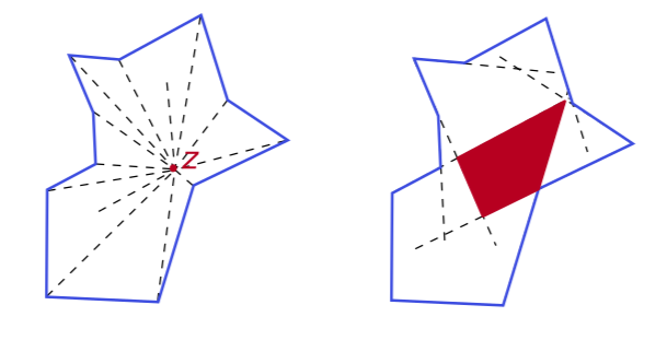
The image above shows an example in 2D.
- On the left we see an irregular non-convex closed polygon where a kernel point is shown along with the lines that connect it to all other vertices.
- On the right we now show its visibility kernel in red, that is the set of all kernel points. Also, it is important to note that the kernel may be computed by simply taking the intersection of all inner half-planes defined by each face, i.e. the half-planes of each face whose normal vector points to the inside of the shape.
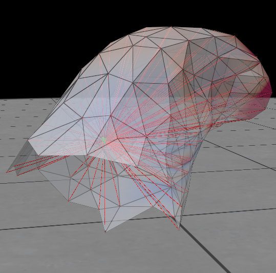
As a 3D example, we shown in the image bellow a 3D mesh of the tip of a thumb, where we can see a green point inside the mesh (a kernel point) from which red lines are drawn to every vertex of the mesh.
Point Sampling
Before we explore the 2 approaches (interior and surface), we first go about finding sample points on the mesh from which to grow the regions. These can be both interior and surface points.
Surface points
To sample points on a 3D surface, several strategies exist, each with distinct advantages. The most common approaches are:
Uniform Sampling: This is the most straightforward method, aiming to distribute points evenly across the surface area of the mesh. It typically works by selecting points randomly, with the probability of selection being proportional to the area of the mesh’s faces. While simple and unbiased, this approach is “blind” to the actual geometry, meaning it can easily miss small but important features like sharp corners or fine details.
Curvature Sampling: This is a more intelligent, adaptive approach that focuses on capturing a shape’s most defining characteristics. The core idea is to sample more densely in regions of high geometric complexity. These areas, often called “interest points,” are identified by their high curvature values, such as Gaussian curvature (\(\kappa_G\)) or mean curvature (\(\kappa_H\)). By prioritizing these salient features (corners, edges, and sharp curves), this method produces a highly descriptive set of sample points that is ideal for creating robust shape descriptors for matching and analysis.
Farthest-Point Sampling (FPS): This iterative algorithm is designed to produce a set of sample points that are maximally spread out across the entire surface. The process is as follows:
- A single starting point is chosen randomly.
- The next point selected is the one on the mesh that has the greatest geodesic distance (the shortest path along the surface) to the first point.
- Each subsequent point is chosen to be the one farthest from the set of all previously selected points.
This process is repeated until the desired number of samples is reached.
In this project we implemented the curvature and FPS methods. However, none of these approaches gave us the desired distribution of points. So we came up with a hybrid approach: Farthest-Point Curvature-Informed sampling (FPCIS) . It aims to achieve a balance between two competing goals:
- Coverage: The sampled points should be spread out evenly across the entire surface, avoiding large unsampled gaps. This is the goal of the standard Farthest Point Sampling (FPS) algorithm.
- Feature-Awareness: The sampled points should be located at or near geometrically significant features, such as sharp edges, corners, or deep indentations. This is where curvature comes into play.
We start by selecting the highest curvature point in the mesh. Then, similar to FPS we compute the geodesic distances from this selected point to all other points using the Dijkstra algorithm over the mesh. However, instead of just taking the farthest point, we first create a pool of the top 30% farthest points, and from this pool we then select the one with highest curvature. The subsequent points are chosen in a similar manner to FPS.
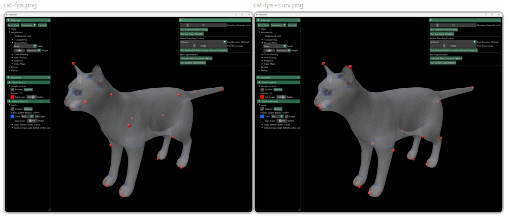
The image above shows the sampling of 15 points using pure FPS (left) and using the FPCIS (right). we see that although FPS gives a pretty well distributed set of sample points we found that some regions that we deemed important where being left out. For example, when sampling 15 points using FPS on the cat model one of the ears was not being sampled. When using the curvature-informed approach we can see that the important regions are correctly sampled.
Interior points
To achieve a list of points that lie well inside the mesh and have good visibility out to the surface, we cast rays inward from every face and recording where they first hit the opposite side of the mesh. Concretely:
- For each triangular face, we compute its centroid.
- We flip the standard outward face normal to get an inward direction \(d\).
- From each centroid, we cast a ray along \(d\), offset by a tiny \(\epsilon\) so it doesn’t immediately self‐intersect.
- We use the Möller–Trumbore algorithm to find the first triangle hit by each ray.
- The midpoint between the ray origin and its first intersection point becomes one of our skeletal nodes—a candidate interior sample.
Casting one ray per face can produce thousands of skeletal nodes. We apply two complementary down‐sampling techniques to reduce this to a few dozen well‐distributed guards:
- Euclidean Farthest Point Sampling (FPS)
- Start from an arbitrary seed node.
- Iteratively pick the next node that maximizes the minimum Euclidean distance to all previously selected samples.
- This spreads points evenly over the interior “skeleton” of the mesh.
- k-Means Clustering
- Cluster all the midpoints into k groups via standard k-means in \(\mathbb R^3\).
- Use each cluster centroid as a down‐sampled guard point.
- This tends to place more guards in densely populated skeleton regions while still covering sparser areas.
Interior Approach
Building upon the interior points sampled earlier, Yu & Li (2011) proposed 2 methods to decompose the mesh into star-shaped pieces: Greedy and Optimal.
1. Greedy Strategy
To achieve this, we solve a fast set-cover heuristic:
Repeatedly pick the guard whose visible-face set covers the most currently uncovered faces, remove those faces, and repeat until every face is covered.
- For each guard \(g\), we shoot one ray per face-centroid to decide which faces it can “see.” We store these as sets
$$ C_j=\{i: \text{face i is visible from } g_j\}$$ - Let \(U = { 0,1,…, |F|−1}\) be the set of all uncovered faces.
- Repeat the following steps until \(U\) is empty:
- For each guard j, compute the number of new faces it would cover:
$$ s_j = | C_j \cap U | $$ - Pick the guard j with the largest \(s_j\).
- Record one star-patch of size \(s_j\).
- Remove those faces: \(U = U \backslash C_j\).
- For each guard j, compute the number of new faces it would cover:
- Output: Get a list of guard indices (= number of star-shaped pieces) that covers the entire mesh.
2. Optimal Strategy
To get the fewest possible star-pieces from the pre-determined finite set of candidate guards, we cast the problem exactly as a minimum set-cover integer program:
- Decision variables: Introduce binary \(x_j \in \{0,1\}\) for each guard \(g_j\).
- Every face i must be covered by at least one selected guard (constraint) and we aim to minimize the total number of guards (thus pieces), hence together we solve:
The overall pipeline of our implementation is as follows:
- We build the \(|F| \times L\) visibility matrix in sparse COO format.
- We feed it to SciPy’s
milp, wrapping the “≥1” rows in aLinearConstraintand all variables as binary in a singleBoundsobject. - The solver returns the provably optimal set of \(x_j\). The optimization problem can be stated as \(\min \sum_{i=1}^m x_i\) subject to \(x_i=0,1\) and \(\sum_{j\in J(i)} x_j\ge 1, \forall i\in\{1,\dots,n\}\).
Experimental Results
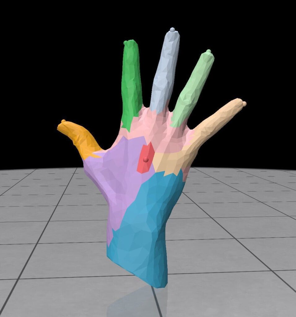
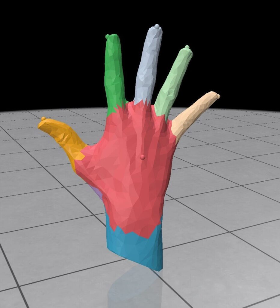
We ran both methods on a human hand mesh with 1515 vertices and 3026 faces. The results are shown below:
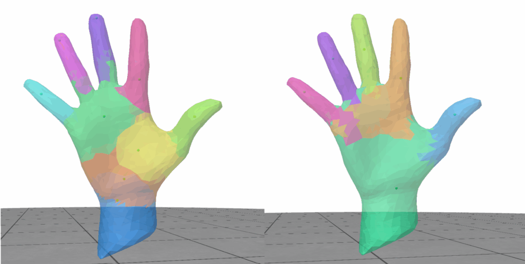
| Down-sampling method | Strategy | # of candidate guards | # of star-shaped pieces | Piece connectivity |
| FPS sampling | Greedy | 25 | 13 | No |
| 50 | 9 | Yes | ||
| Optimal | 25 | 9 | No | |
| 50 | 6 | No | ||
| K-means clustering | Greedy | 25 | 8 | No |
| 50 | 8 | No | ||
| Optimal | 25 | 7 | No | |
| 50 | 6 | No |
Some key observations are:
- Both interior approaches have no constraints to ensure connectivity among faces of the same guard, hence causing difficulties in closing the mesh of each piece or inaccurate calculation of final connected piece number.
- Down-sampling methods: k‐means clustering tends to slightly better distribute guards in high‐density skeleton regions, hence having a smaller gap between greedy and optimal strategy.
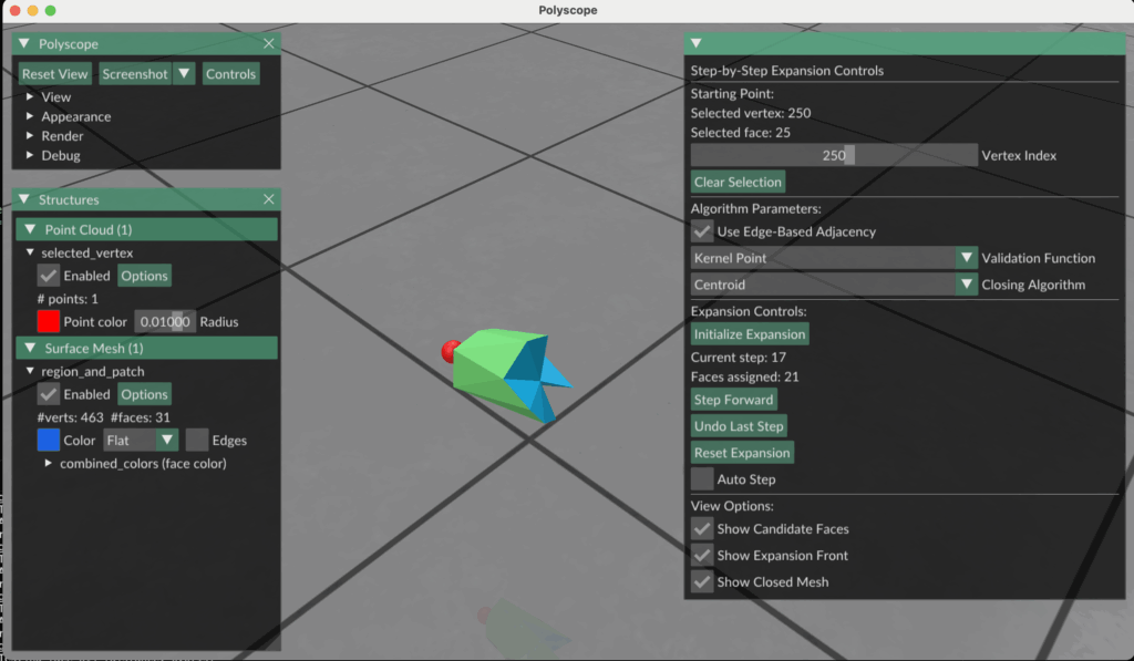
Surface Approach: Surface-Guided Growth with Mesh Closure
One surface-based strategy we explored is a region-growing method guided by local surface connectivity and kernel validation, with explicit mesh closure at each step. The goal is to grow star-shaped regions from sampled points, ensuring at every expansion that the region remains visible from at least one interior point.
This method operates in parallel for each of the N sampled seed points. Each seed initiates its own region and grows iteratively by considering adjacent faces.
Expansion Process
- Initialization:
- Begin with the seed vertex and its immediate 1-ring neighborhood—i.e., the three faces incident to the sampled point.
- Iterative Expansion:
- Identify all candidate faces adjacent to the current region (i.e., faces sharing an edge with the region boundary).
- Sort candidates by distance to the original seed point.
- For each candidate face:
- Temporarily add the face to the region.
- Close the region to form a watertight patch using one of the following mesh-closing strategies:
- Centroid Fan – Connect boundary vertices to their centroid to create triangles.
- 2D Projection + Delaunay – Project the boundary to a plane and apply a Delaunay triangulation.
- Run a kernel visibility check: determine if there exists a point (the kernel) from which all faces in the current region + patch are visible.
- If the check passes, accept the face and continue.
- If not, discard the face and try the next closest candidate.
- If no valid candidates remain, finalize the region and stop its expansion.
Results and Conclusions
- The kernel check was not robust enough—some regions were allowed to grow into areas that clearly violated visibility constraints.
- Region boundaries could expand too aggressively, reaching parts of the mesh that shouldn’t logically belong to the same star-shaped segment.
- Small errors in patch construction led to instability in the visibility test, particularly for thin or highly curved regions.
As such, the final segmentations were often overextended or incoherent, failing to produce clean, usable star regions. Despite these issues, this approach remains a useful prototype for purely surface-based decomposition, offering a baseline for future improvements in kernel validation and mesh closure strategies.

References
Steffen Hinderink, Hendrik Brückler, and Marcel Campen. (2024). Bijective Volumetric Mapping via Star Decomposition. ACM Trans. Graph. 43, 6, Article 168 (December 2024), 11 pages. https://doi.org/10.1145/3687950
Yu, W. and Li, X. (2011), Computing 3D Shape Guarding and Star Decomposition. Computer Graphics Forum, 30: 2087-2096. https://doi.org/10.1111/j.1467-8659.2011.02056.x
Yusuf Sahillioğlu. “digital geometry processing – mesh comparison.” YouTube Video, 1:11:26. April 30, 2020. https://www.youtube.com/watch?v=ySr54PMAlGo.