Categories
Research

Topology Control: Pathfinding for Genus Preservation (2/2)

SGI Fellows:
Stephanie Atherton, Marina Levay, Ualibyek Nurgulan, Shree Singhi, Erendiro Pedro

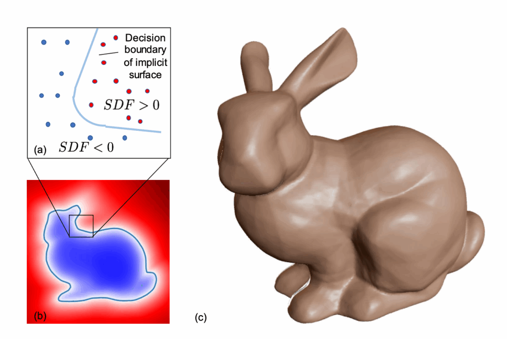
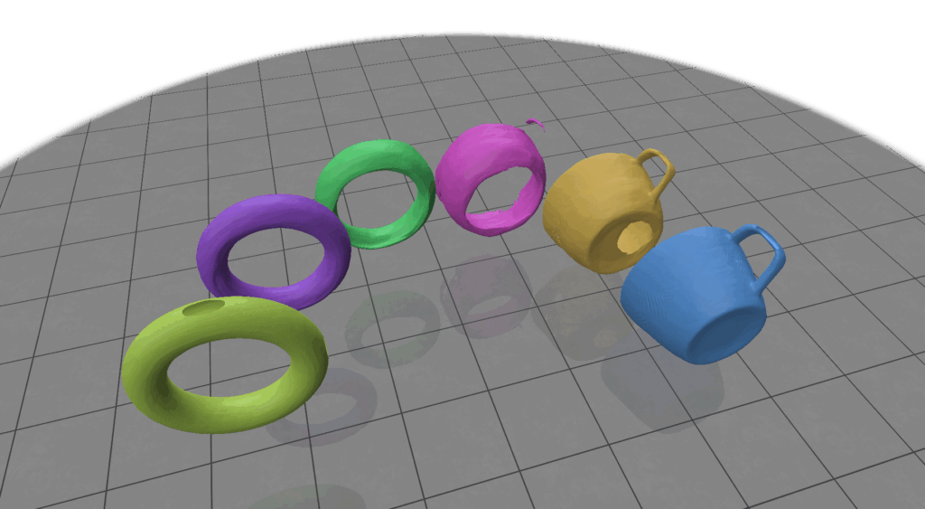
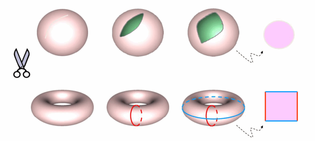
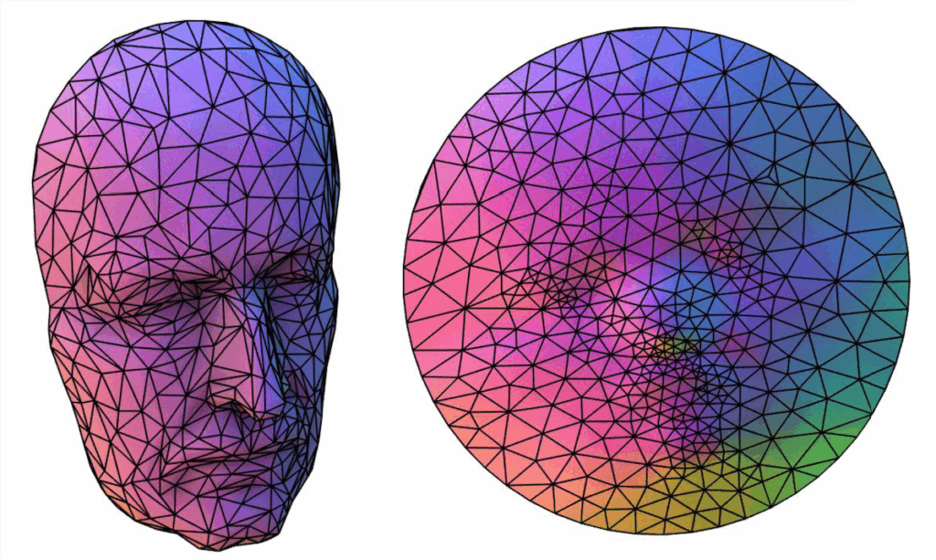
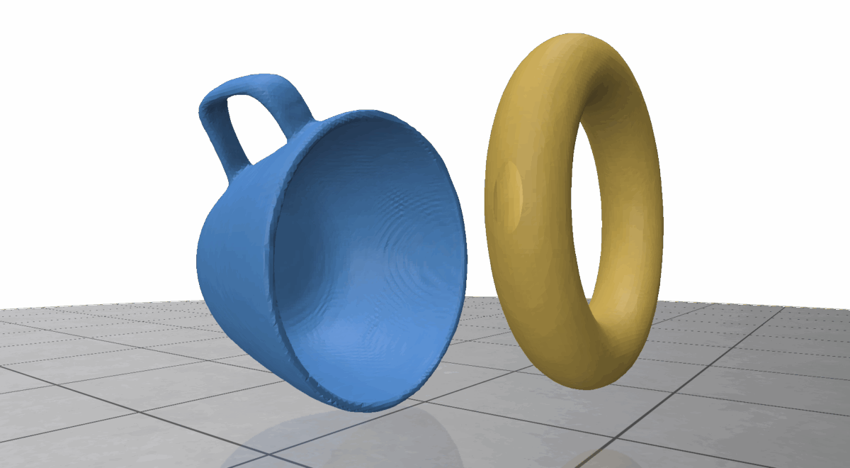
Recall (from post 1/2) that while DeepSDFs are a powerful shape representation, they are not inherently topology-preserving. By “preserving topology,” we mean maintaining a specific topological invariant throughout shape deformation. In low-dimensional latent spaces \(z_{\text{dim}} = 2\), linear interpolation between two topologically similar shapes can easily stray into regions with a different genus, breaking that invariant.

Visualizing genera count in 2D latent space

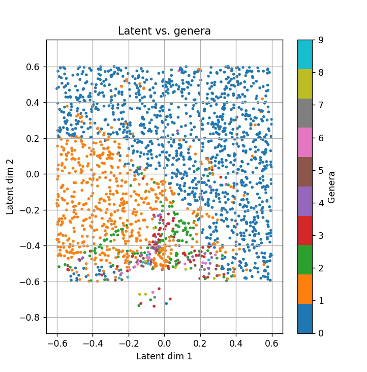
Higher-dimensional latent spaces may offer more flexibility—potentially containing topology-preserving paths—but these are rarely straight lines. This points to a broader goal: designing interpolation strategies that remain within the manifold of valid shapes. Instead of naive linear paths, we focus on discovering homotopic trajectories—routes that stay on the learned shape manifold while preserving both geometry and topology. In this view, interpolation becomes a trajectory-planning problem: navigating from one latent point to another without crossing into regions of invalid or unstable topology.

Pathfinding in Latent Space

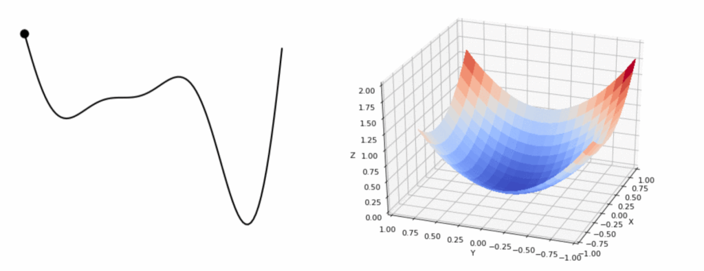
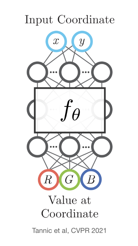
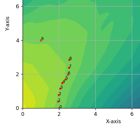
Suppose you are a hiker hoping to a reach a point \(A\) from a point \(B\) amidst a chaotic mountain range. Now your goal is to plan your journey so that there will be minimal height change in your trajectory, i.e., you are a hiker that hates going up and down much! Fortunately, an oracle gives us a magical device, let us call it \(f\), that can give us the exact height of any point we choose. In other words, we can query \(f(x)\) for any position \(x\), and this device is differentiable, \(f'(x)\) exists!

Metaphors aside, the problem of planning a path from a particular latent vector \(A\) to another \(B\) in the learned latent space would greatly benefit from another auxiliary network that learns the mapping from the latent vectors to the desired topological or geometric features. We will introduce a few ways to use this magical device – a simple neural network.

Gradient as the Compass

Now the best case scenario would be to stay at the same height for the whole of the journey, no? This greedy approach puts a hard constraint on the problem, but it also greatly reduces the possible space of paths to take. For our case, we would love to move toward the direction that does not change our height, and this set of directions precisely forms the nullspace of the gradient.

No height change in mathematical terms means that we look for directions where the derivatives equal zero, as in

$$D_vf(x) = \nabla f(x)\cdot v = 0,$$


where the first equality is a fact of the calculus and the second shows that any desirable direction \(v\in \text{null}(\nabla f(x))\).

This does not give any definitive directions for a position \(x\) but a set of possible good directions. Then a greedy approach is to take the direction that aligns most with our relative position against the goal – the point \(B\).

Almost done, but the problem is that if we always take steps with the assumption that we are on the correct isopath, we would end up accumulating errors. So, we actually want to nudge ourselves a tiny bit along the gradient to land back on the isopath. Toward this, let \(x\) be the current position and \(\Delta x=\alpha \nabla f(x) + n\), where \(n\) is the projection of \(B-x\) to \(\text{null}(\nabla f(x))\). Then we want \(f(x+\Delta x) = f(B)\). Approximate

$$f(B) = f(x+\Delta x) \approx f(x) + \nabla f(x)\cdot \Delta x,$$

and substituting for \(\Delta x\), see that

$$f(x) + \nabla f(x) \cdot (\alpha\nabla f(x) + n) \
\Longleftrightarrow
\alpha \approx \frac{f(B) – f(x)}{|\nabla f(x)|^2}.$$

Now we just take \(\Delta x = \frac{f(B) – f(x)}{|\nabla f(x)|^2}\nabla f(x) + \text{proj}_{\text{null}(\nabla f(x))} (B- x)\) for each position \(x\) on the path.

Results. Latent to expected volume.

Optimizing Vertical Laziness

Sometimes it is impossible to hope for the best case scenario. Even when \(f(A)=f(B)\), it might happen that the latent space is structured such that \(A\) and \(B\) are in different components of the level set of the function \(f\). Then there is no hope for a smooth hike without ups and downs! But the situation is not completely hopeless if we are fine with taking detours as long as such undesirables are minimized. We frame the problem as

$$\text{argmin}_{x_i \in L, \forall i} \sum_{i=1}^n |f(x_i) – f(B)|^2 + \lambda\sum_{i=1}^{n-2} |(x_{i+2}-x_{i+1}) – (x_{i+1} – x_i)|^2,
$$

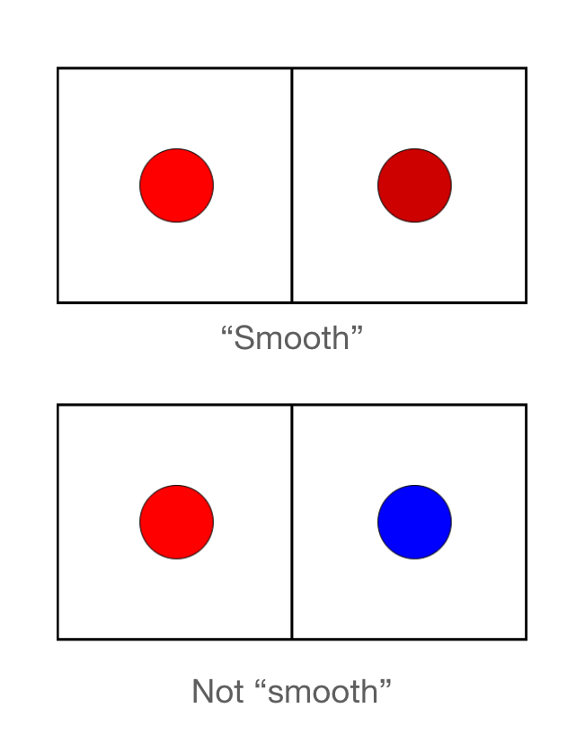
where \(L\) is the latent space and \({x_i}_{i=1}^n\) is the sequence defining the path such that \(x_1 = A\) and \(x_n=B\). The first term is to encourage consistency in the function values, while the second term discourages sudden changes in curvature, thereby ensuring smoothness. Once defined, various gradient-based optimization algorithms can be used on this problem, which is now imposed with a relatively soft constraint.

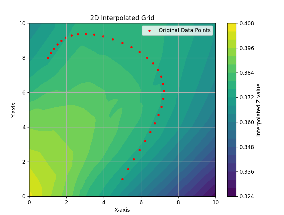
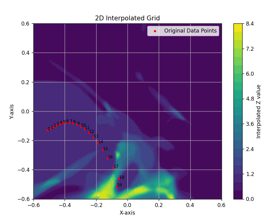
Results of pathfinding via optimization in different contexts.

Latent to expected volume.
Latent to expected genus.

A Geodesic Path

One alternative attempt of note to optimize pathfinding used the concept of geodesics, or the shortest, smoothest distance between two points on a Riemannian manifold. In the latent space, one is really working over a latent data manifold, so thinking geometrically, we experimented with a geodesic path algorithm. In writing this algorithm, we set our two latent endpoints and optimized the points in between by minimizing the energy of our path on the output manifold. This alternative method worked similarly well to the optimized pathfinding algorithm posed above!

Conclusion and Future Work

Our journey into DeepSDFs, gradient methods, and geodesic paths has shown both the promise and the pitfalls of blending multiple specialized components. The decoupled design gave us flexibility, but also revealed a fragility—every part must share the same initialized latent space, and retraining one element (like the DeepSDF) forces a retraining of its companions, the regressor and classifier. With each component carrying its own error, the final solution sometimes felt like navigating with a slightly crooked compass.

Yet, these challenges are also opportunities. Regularization strategies such as Lipschitz constraints, eikonal terms, and Laplacian smoothing may help “tame” topological features, while alternative frameworks like diffeomorphic flows and persistent homology could provide more robust topological guarantees. The full integration of these models remains a work in progress, but we hope that this exploration sparks new ideas and gives you, the reader, a sharper sense of how topology can be preserved—and perhaps even mastered—in complex geometric learning systems.

Genus is a commonly known and widely applied shape feature in 3D computer graphics, but there is also a whole mathematical menu of topological invariants to explore along with their preservation techniques! Throughout our research, we also considered:

  • Would topological accuracy benefit from a non-differentiable algorithm (e.g. RRT) that can directly encode genus as a discrete property? How would we go about certifying such an algorithm?
  • How can homotopy continuation be used for latent space pathfinding? How will this method complement continuous deformations of homotopic and even non-homotopic shapes?
  • What are some use cases to preserve topology, and what choice of topological invariant should we pair with those cases?

We invite all readers and researchers to take into account our struggles and successes in considering the questions posed.

Acknowledgements. We thank Professor Kry for his mentorship, Daria Nogina and Yuanyuan Tao for many helpful huddles, Professor Solomon for his organization of great mentors and projects, and the sponsors of SGI for making this summer possible.

References

DeepSDF

SDFConnect

Categories
Research

Topology Control: Training a DeepSDF (1/2)

SGI Fellows:
Stephanie Atherton, Marina Levay, Ualibyek Nurgulan, Shree Singhi, Erendiro Pedro

In the Topology Control project mentored by Professor Paul Kry and project assistants Daria Nogina and Yuanyuan Tao, we sought to explore preserving topological invariants of meshes within the framework of DeepSDFs. Deep Signed Distance Functions are a neural implicit representation used for shapes in geometry processing, but they don’t come with the promise of respecting topology. After finishing our ML pipeline, we explored various topology-preserving techniques through our simple, initial case of deforming a “donut” (torus) into a mug.

DeepSDFs

Signed Distance Field (SDF) representation of a 3D bunny. The network predicts the signed distance from each spatial point to the surface. Source: (Park et al., 2019).

Signed Distance Functions (SDFs) return the shortest distance from any point in 3D space to the surface of an object. Their sign indicates spatial relation: negative if the point lies inside, positive if outside. The surface itself is defined implicitly as the zero-level set: the locus where \(\text{SDF}(x) = 0 \).

In 2019, Park et al. introduced DeepSDF, the first method to learn a continuous SDF directly using a deep neural network (Park et al., 2019). Given a shape-specific latent code \( z \in \mathbb{R}^d \) and a 3D point \( x \in \mathbb{R}^3 \), the network learns a continuous mapping:

$$
f_\theta(z_i, x) \approx \text{SDF}^i(x),
$$

where \( f_\theta \) takes a latent code \( z_i \) and a 3D query point \( x \) and returns an approximate signed distance.

The training set is defined as:

$$
X := {(x, s) : \text{SDF}(x) = s}.
$$

Training minimizes the clamped L1 loss between predicted and true distances:

$$
\mathcal{L}\bigl(f_\theta(x), s\bigr)
= \bigl|\text{clamp}\bigl(f_\theta(x), \delta\bigr) – \text{clamp}(s, \delta)\bigr|
$$

with the clamping function:

$$
\text{clamp}(x, \delta) = \min\bigl(\delta, \max(-\delta, x)\bigr).
$$

Clamping focuses the loss near the surface, where accuracy matters most. The parameter \( \delta \) sets the active range.

This is trained on a dataset of 3D point samples and corresponding signed distances. Each shape in the training set is assigned a unique latent vector \( z_i \), allowing the model to generalize across multiple shapes.

Once trained, the network defines an implicit surface through its decision boundary, precisely where \( f_\theta(z, x) = 0 \). This continuous representation allows smooth shape interpolation, high-resolution reconstruction, and editing directly in latent space.

Training Field Notes

We sampled training data from two meshes, torus.obj and mug.obj using a mix of blue-noise points near the surface and uniform samples within a unit cube. All shapes were volume-normalized to ensure consistent interpolation.

DeepSDF is designed to intentionally overfit. Validation is typically skipped. Effective training depends on a few factors: point sample density, network size, shape complexity, and sufficient epochs.

After training, the implicit surface can be extracted using Marching Cubes or Marching Tetrahedra to obtain a polygonal mesh from the zero-level set.

Training Parameters
SDF Delta1.0
Latent Mean0.0
Latent SD0.01
Loss FunctionClamped L1
OptimizerAdam
Network Learning Rate0.001
Latent Learning Rate0.01
Batch Size2
Epochs5000
Max Points per Shape3000
Network Architecture
Latent Dimension16
Hidden Layer Size124
Number of Layers8
Input Coordinate Dim3
Dropout0.0
Point Cloud Sampling
Radius0.02
Sigma0.02
Mu0.0
Number of Gaussians10
Uniform Samples5000

For higher shape complexity, increasing the latent dimension or training duration improves reconstruction fidelity.

Latent Space Interpolation

One compelling application is interpolation in latent space. By linearly blending between two shape codes \( z_a \) and \( z_b \), we generate new shapes along the path

$$
z(t) = (1 – t) \cdot z_a + t \cdot z_b,\quad t \in [0,1].
$$

Latent space interpolation between mug and torus.

While DeepSDF enables smooth morphing between shapes, it exposes a core limitation: a lack of topological consistency. Even when the source and target shapes share the same number of genus, interpolated shapes can exhibit unintended holes, handles, or disconnected components. These are not artifacts, they reveal that the model has no built-in notion of topology.

However, this limitation also opens the door for deeper exploration. If neural fields like DeepSDF lack an inherent understanding of topology, how can we guide them toward preserving it? In the next post, we explore a fundamental topological property—genus—and how maintaining it during shape transitions could lead us toward more structurally meaningful interpolations.

References

Categories
Tutorial week

Tutorial Week Day 4: Texture Optimization

Intro

Now that you’ve gotten the grasp of meshes, and created your very first 3D object on Polyscope, what can we do next? On Day 4 of the SGI Tutorial Week, we had speakers Richard Liu and Dale Decatur from the Threedle Lab at UChicago explaining about Texture Optimization.

In animated movies and video games, we are used to observing them with realistic textures. Intuitively, we might imagine that we have this texture as a map applied as a flat “sticker” over it. However, we know from some well-known examples in cartography that it is difficult to create a 2D map of a 3D shape like the Earth without introducing distortions or cuts.

Besides, ideally, we would want to be able to transition from the 2D to the 3D map interchangeably. Framing this 2D map as a function on \(\mathbb{R^2}\), we would like it to be bijective.

The process of creating a bijective map from a mesh S in \(\mathbb{R^3}\) to a given domain \(\Omega\), or \(F: \Omega \leftrightarrow S\), is known as mesh parametrization.

UV Unwrapping

Consider a mesh defined by the object as \(M = {V, E, F}\), with Vertices, Edges and Faces respectively, where:

\begin{equation*} V \subset R^3 \end{equation*} \begin{align*} E = \{(i, j) \quad &| \text{\quad vertex i is connected to vertex j}\} \\ F = \{(i, j, k) \quad &| \quad \text{vertex i, j , k share a face}\} \end{align*}

For a mesh M, we define the parametrization as a function mapping vertices \(V\) to some domain \(\Omega\)

\begin{equation*} U: V \subset \mathbb{R}^3 \rightarrow \Omega \subset \mathbb{R}^2 \end{equation*}

For every vertex \(v_i\) we assign a 2D coordinate \(U(v_i) = (u_i, v_i)\) (this is why the method is called UV unwrapping).

This parametrization has a constraint, however. Only disk topology surfaces (those with a 1 boundary loop) surfaces admit a homeomorphism (a continuous and bijective map) to the bounded 2D plane.

Source: Richard Liu

As a workaround, we can always introduce a cut.

Source: Richard Liu

However, these seams create discontinuities, and in turn, distortions we want to minimize. We can distinguish different kinds of distortions using the Jacobian, the matrix of all first-order partial derivatives of a vector-valued function. Specifically, we look at the singular values of the Jacobian (which in the UV function is defined as a 2×3 matrix per triangle).

\begin{align*} J_f = U\Sigma V^T = U \begin{pmatrix} \sigma_1 & 0 \\ 0 & \sigma_2 \\ 0 & 0 \end{pmatrix} V^T \\ f \text{ is equiareal or area preserving} \Leftrightarrow \sigma_1 \sigma_2 &= 1 \\ f \text{ is equiareal or area preserving} \Leftrightarrow \sigma_1 &= \sigma_2 \\ f \text{ is equiareal or area preserving} \Leftrightarrow \sigma_1 &= \sigma_2 = 1 \end{align*}

We can find the Jacobians of the UV map assignment \(U\) using the mesh gradient operator \(G \in \mathbb{R}^{3|F|\times V}\)

\begin{align*} GU = J \in \mathbb{R}^{3|F|\times V} \end{align*}

The classical approach for optimizing a mesh parametrization is viewing the mesh surface as the graph of a mass-spring system (least squares optimization problem). The mesh vertices are the nodes (with equal mass) with each edge acting as a spring with some stiffness constant.

Source: Richard Liu

Two key design choices in setting up this problem are:

  • Where to put the boundary?
  • How to set the spring weights (stiffness)?

To compute the parametrization, we minimize the sum of spring potential energies.

\begin{align*} \min_U \sum_{\{i, j\} \in E} w_ij || u_i – u_j||^2 \end{align*}

Where \(u_i = (u_i, v_i)\) is the UV coordinate to vertex i. We then aim to solve the ODE:

\begin{align*} \frac{\partial E}{\partial u _i }= \sum_{j \in N_i} 2 \cdot w_{ij} (u_i – u_j) = 0 \end{align*}

Where \(N_i\) indexes all neighbors of vertex \(i\). We can now fix the boundary vertices and solve each equation for the remaining \(u_i\).

A solution by Tutte (1963) and Floater (1997) was computed such that if the boundary is convex and the weights are positive, the solution is guaranteed to be injective. While an injective map has its limitations in terms of transferring the texture back into the 3D shape, it allows us to easily visualize the 2D map of this shape.

Here, we would need to fix or map a boundary to a circle, where all weights are 1.

An alternative to the classical approach is trivial parametrization, where we split the mesh up into its individual triangles in a triangle soup and then flatten each triangle (isometric distortion). We would then translate and scale all triangles to be packed into the unit square.

Source: Richard Liu

Translation and uniform scaling does not affect the angles, such that we have no angle distortion. So this tells us that this parametrization approach is conformal.

Still, when packing triangles into the texture image, we might need to rescale them so they fit, meaning the areas are not guaranteed to be the same. We can verify this based on the SDF values:

\begin{align*} \sigma_1\sigma_2 \neq 1 \end{align*}

This won’t be too relevant in the end though because all triangles get scaled by the same factor, so that the area of each triangle is preserved up to some global scaler. As a result, we would still get an even sampling of the surface, which is what we would care about, at least intuitively, for texture mapping.

However, applying a classical algorithm to trivial parametrization is typically a bad solution because it introduces maximal cuts (discontinuities). How can we overcome this issue?

Parametrization with Neural Networks

Assume we have some parametrized function and some target value. With an adaptive learning algorithm, we determine the direction in which to change our parameters so that the function moves closer to our target.

We compute some loss or measure of closeness between our current function evaluation and our target value.We then compute the gradient of this loss with respect to our parameters. Take a small step in that direction. We would repeat this process until we ideally achieved the global minimum.

Source (left) and Source (right)

Similarly, we can use an approach to optimize the mesh texture.

  • Parametric function = rendering function
  • Parameters = texture map pixel values (texel = texture pixel)
  • Target = existing images of the object with the desired colors
  • Loss = pixel differences between our rendered images and target images.

What happens if we do this? We do achieve a texture map, but each pixel is mostly optimized independently. As a result, the texture ends up more grainy.

Source: Dale Decatur

Improving Smoothness

What can we do to improve this? Well, we would want to make the function more smooth. For this, we can optimize a new function \(\phi(u, v) : \mathbb{R}^2 \rightarrow \mathbb{R}^2\) that maps the texels to RGB color values. By smoothness in \(\phi\), we mean that \(\phi\) is continuous.

To get the color at any point in the 2D texture map, we just need to query \(\phi\) at that UV coordinate!

Source: Dale Decatur

To encourage smoothness in \(\phi\), we can use a 3D coordinate network.


Tannic et al, CVPR 2021

Consider a mapping from a 3D surface to a 2D texture. We can learn a 3D coordinate \(\phi\): \(\mathbb{R}^3 \rightarrow \mathbb{R}^2\) that maps 3D surface points to RGB colors. \(\phi(x, y, z) = (R, G, B)\).

We can then use the inverse map to go from 2D texture coordinates to 3D surface points, then query those points with the coordinate network to get colors, then map those colors back to the 2D texture for easy rendering.

Source: Dale Decatur

How to compute an inverse map?

We aim to have a mapping from texels to surface poitns, but we already have a mapping from the vertices to the texel plane. The way we can map an arbitrary coordinate to the surface is through barycentric interpolation, a coordinate system relative to a given triangle. In this system, any points has 3 barycentric coordinates.