SGI Fellows: Haojun Qiu, Nhu Tran, Renan Bomtempo, Shree Singhi and Tiago Trindade Mentors: Sina Nabizadeh and Ishit Mehta SGI Volunteer: Sara Samy
Introduction
The field of Computational Fluid Dynamics (CFD) has long been a cornerstone of both stunning visual effects in movies and video games, and also a critical tool in modern engineering, for designing more efficient cars and aircrafts for example. At the heart of any CFD application there exists a solver that essentially predicts how a fluid moves in space at discrete time intervals. The dynamic behavior of a fluid is governed by a famous set of partial differential equations, called the Navier-Stokes equations, here presented in vector form:
where \(t\) is time, \(\mathbf{u}\) is the varying velocity vector field, \(\rho\) is the fluids density, \(p\) is the pressure field, \(\nu\) is the kinematic viscosity coefficient and \(\mathbf{f}\) represents any external body forces (e.g. gravity, electromagnetic, etc.). Let’s quickly break down what each term means in the first equation, which describes the conservation of momentum:
\(\dfrac{\partial \mathbf{u}}{\partial t}\) is the local acceleration, describing how the velocity of the fluid changes at a fixed point in space.
\((\mathbf{u} \cdot \nabla) \mathbf{u}\) is the advection (or convection) term. It describes how the fluid’s momentum is carried along by its own flow. This non-linear term is the source of most of the complexity and chaotic behavior in fluids, like turbulence.
\(\frac{1}{\rho}\nabla p\) is the pressure gradient. It’s the force that causes fluid to move from areas of high pressure to areas of low pressure.
\(\nu \nabla^{2} \mathbf{u}\) is the viscosity or diffusion term. It accounts for the frictional forces within the fluid that resist flow and tend to smooth out sharp velocity changes. For the “Gaussian Fluids” paper, this term is ignored (\(\nu=0\)) to model an idealized inviscid fluid.
The second equation, \(\nabla \cdot \mathbf{u} = 0\), is the incompressibility constraint. It mathematically states that the fluid is divergence-free, meaning it cannot be compressed or expanded.
The first step to numerically solving these equations on some spatial domain \(\Omega\) using classical solvers is to discretize this domain. To do that, two main approaches have dominated the field from its very beginning:
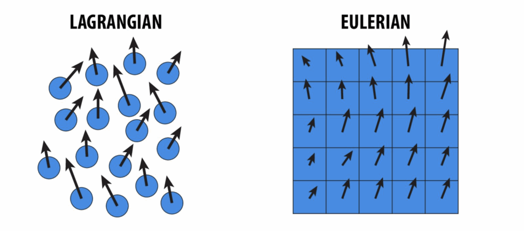
Eulerian methods: which use fixed grids that partition the spatial domain into a (un)structured collection of cells on which the solution is approximated. However, these methods often suffer from “numerical viscosity,” an artificial damping that smooths away fine details;
Lagrangian methods: which use particles to sample the solution at certain points in space and that move with the fluid flow. However, these methods can struggle with accuracy and capturing delicate solution structures.
The core problem has always been a trade-off. Achieving high detail with traditional solvers often requires a massive increase in memory and computational power, hitting the “curse of dimensionality”. Hybrid Lagrangian-Eulerian methods that try to combine the best of both worlds can introduce their own errors when transferring data between grids and particles. The quest has been for a representation that is expressive enough to capture the rich, chaotic nature of fluids without being computationally prohibitive.
A Novel Solution: Gaussian Spatial Representation
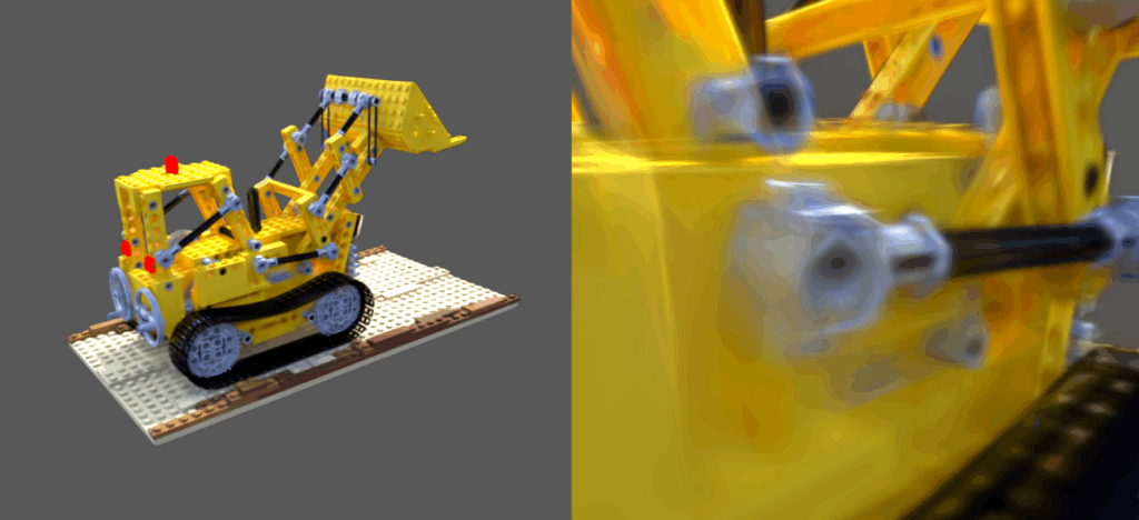
By now you have probably come across an emerging technology in the field of 3D rendering called 3D Gaussian Splatting (3DGS). It attempts to represent a 3D scene using, not traditional polygonal meshes or volumetric voxels, but in a manner similar to an artist using paint brush strokes to approximate a colored picture, Gaussian Splatting uses 3D gaussians to “paint” a 3D scene. These gaussians are nothing more than a ellipsoid with a color value and opacity associated.
Think of each Gaussian not as a solid, hard-edged ellipsoid, but as a soft, semi-transparent cloud (Fig.2). It’s most opaque and dense at its center and it smoothly fades to become more transparent as you move away from the center. The specific shape, size, and orientation of this “cloud” are controlled by its parameters. By blending thousands or even millions of these colored, transparent splats together, Gaussian Splatting can represent incredibly detailed and complex 3D scenes.
Fig.1 Example 3DGS of a Lego build (left) and a zoomed in view of the gaussians that make it up (right).
Drawing from this incredible effectiveness of using gaussians to encode complex geometry and lighting of 3D scenes, a new paper presented at SIGGRAPH 2025 titled “Gaussian Fluids: A Grid-Free Fluid Solver based on Gaussian Spatial Representation” by Jingrui Xing et al. introduces a fascinating new approach to computational domain representation for CFD applications.
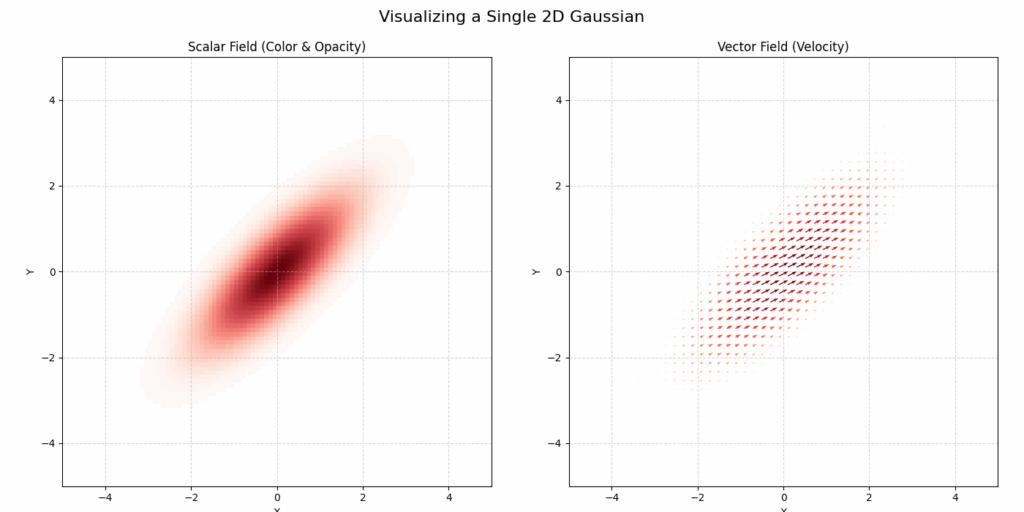
The new method, named Gaussian Spatial Representation (GSR), uses gaussians to essentially “paint” vector fields. While 3DGS encodes local color information into each gaussian, GSR encodes local vector fields. In this way each gaussian stores a vector that defines a local direction of the velocity field, where the magnitude of the vectors is greater closer the gaussian’s center, and quickly gets smaller when moving farther from it. In Fig.2 we can see an example of 2D gaussian viewed with color data (left), as well as with a vector field (right).
Fig.2 Example plot of a 2D Gaussian with scalar data (left) and vector data (right)
By splatting a lot of these gaussians and adding the vectors we can then define a continuously differentiable vector field around a given domain, which allows us to solve the complex Navier-Stokes equations not through traditional discretization, but as a physics-based optimization problem at each time step. A custom loss function ensures the simulation adheres to physical laws like incompressibility (zero-divergence) and, crucially, preserves the swirling motion (vorticity) that gives fluids their character.
Each point represents a Gaussian splat, with its color mapped to the logarithm of its anisotropy ratio. This visualization highlights how individual Gaussians are stretched or compressed in different regions of the domain.
Enforcing Physics Through Optimization: The Loss Functions
The core of the “Gaussian Fluids” method is its departure from traditional time-stepping schemes. Instead of discretizing the Navier-Stokes equations directly, the authors reframe the temporal evolution of the fluid as an optimization problem. At each time step, the solver seeks to find the set of Gaussian parameters that best satisfies the governing physical laws. This is achieved by minimizing a composite loss function, which is a weighted sum of several terms, each designed to enforce a specific physical principle or ensure numerical stability.
Two of the main loss terms are:
Vorticity Loss (\(L_{vor}\)): For a two dimensional ideal (inviscid) fluid, vorticity, defined as the curl of the velocity field (\(\omega=\nabla \times u\)), is a conserved quantity that is transported with the flow. This loss function is designed to uphold this principle. It quantifies the error between the vorticity of the current velocity field and the target vorticity field, which has been advected from the previous time step. By minimizing this term, the solver actively preserves the rotational and swirling structures within the fluid. This is critical for preventing the numerical dissipation (an artificial smoothing of details) that often plagues grid-based methods and for capturing the fine, filament-like features of turbulent flows.
Divergence Loss (\(L_{div}\)): This term enforces the incompressibility constraint, \(\nabla \cdot u=0\). From a physical standpoint, this condition ensures that the fluid’s density remains constant; it cannot be locally created, destroyed, or compressed. The loss function achieves this by evaluating the divergence of the Gaussian-represented velocity field at numerous sample points and penalizing any non-zero values. Minimizing this term is essential for ensuring the conservation of mass and producing realistic fluid motion.
Beyond these two, to function as a practical solver, the system must also handle interactions with boundaries and maintain stability over long simulations. The following loss terms address these requirements:
Boundary Losses (\(L_{b1}\), \(L_{b2}\)): The behavior of a fluid is critically dependent on its interaction with solid boundaries. These loss terms enforce such conditions. By sampling points on the surfaces of geometries within the scene, the loss function penalizes any fluid velocity that violates the specified boundary conditions. This can include “no-slip” conditions (where the fluid velocity matches the surface velocity, typically zero) or “free-slip” conditions (where the fluid can move tangentially to the surface but not penetrate it). This sampling-based strategy provides an elegant way to handle complex geometries without the need for intricate grid-cutting or meshing procedures.
Regularization Losses (\(L_{pos}\), \(L_{aniso}\), \(L_{vol}\)): These terms are included to ensure the numerical stability and well-posedness of the optimization problem.
The Position Penalty (\(L_{pos}\)) constrains the centers of the Gaussians, preventing them from deviating excessively from the positions predicted by the initial advection step. This regularizes the optimization process, improves temporal coherence, and helps prevent particle clustering.
The Anisotropy (\(L_{aniso}\)) and Volume (\(L_{vol}\)) losses act as geometric constraints on the Gaussian basis functions themselves. They penalize Gaussians that become overly elongated, stretched, or distorted. This is crucial for maintaining a high-quality spatial representation and preventing the numerical instabilities that could arise from ill-conditioned Gaussian kernels.
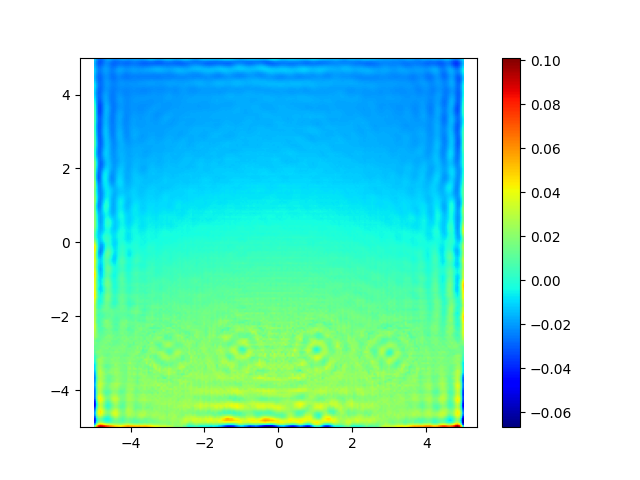
However, when formulating a fluid simulation as a Physics-Based optimization problem, one challenge that soon becomes apparent is that choosing good loss functions can be really tricky. The reliance on “soft constraints”, such as the divergence loss function, in the optimization process means that small errors can accumulate over time. Also, the handling of complex domains with holes (non-simply connected domains) is also a big challenge. When running the Leapfrog simulation we can see that the divergence of the solution, although relatively small, isn’t as close to zero as it should be (ideally it should be exactly zero).
This “Leapfrog” simulation highlights the challenge of “soft constraints.” The “Divergence” plot (bottom-left) shows the small, non-zero errors that can accumulate, while the “Vorticity” plot (bottom-right) shows the swirling structures the solver aims to preserve.
Divergence-free Gaussian Representation
Now we want to extend on this paper a bit. Let’s focus on the 2D case for now. The problem of regularizing divergence is that the velocity vector field won’t be exactly divergence free. I can perhaps help this with an extra step every iteration. Define \(\mathbf{J} \in \mathbb{R}^{2 \times 2}\) as a rotation matrix
This potential function can be constructed with the same gaussian mixture by carrying a \(\phi_{i} \in \mathbb{R}\) at every gaussian, and thus a continuous function having full support
similarly we can replace \(G_i(\mathbf{x})\) with the clamped gaussians \(\tilde{G}_i(\mathbf{x})\) for efficiency. Now we can construct a vector field that is unconditionally divergence-free
and we use the similar approach of Monte Carlo way of sampling \(\mathbf{x}\) uniformly in space.
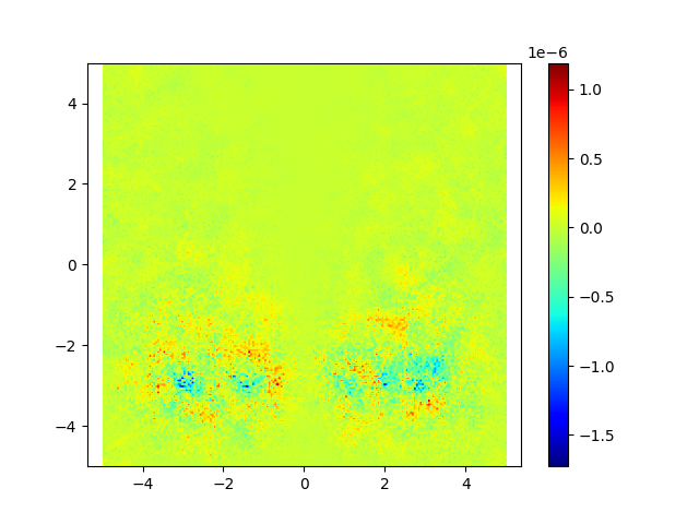
Doing this, we managed to achieve a divergence much closer to zero, as shown in the image below.
Before (left) and after (right)
References
Jingrui Xing, Bin Wang, Mengyu Chu, and Baoquan Chen. 2025. Gaussian Fluids: A Grid-Free Fluid Solver based on Gaussian Spatial Representation. In Proceedings of the Special Interest Group on Computer Graphics and Interactive Techniques Conference Conference Papers (SIGGRAPH Conference Papers ’25). Association for Computing Machinery, New York, NY, USA, Article 9, 1–11. https://doi.org/10.1145/3721238.3730620
SGI Fellows: Lydia Madamopoulou, Nhu Tran, Renan Bomtempo and Tiago Trindade Mentor. Yusuf Sahillioglu SGI Volunteer. Eric Chen
Introduction
In the world of 3D modeling and computational geometry, tackling geometrically complex shapes is a significant challenge. A common and powerful strategy to manage this complexity is to use a “divide-and-conquer” approach, which partitions a complex object into a set of simpler, more manageable sub-shapes. This process, known as shape decomposition, is a classical problem, with convex decomposition and star-shaped decomposition being of particular interest.
The core idea is that many advanced algorithms for tasks like creating volumetric maps or parameterizing a shape are difficult or unreliable on arbitrary models, but work perfectly on simpler shapes like cubes, balls, or star-shaped regions.
The paper by Hinderink et al. (2024) demonstrates this perfectly. It presents a method to create a guaranteed one-to-one (bijective) map between two complex 3D shapes. They achieve this by first decomposing the target shape into a collection of non-overlapping star-shaped pieces. By breaking the hard problem down into a set of simpler mapping problems, they can apply existing, reliable algorithms to each star-shaped part and then stitch the results together. Similarly, the work by Yu & Li (2011) uses star decomposition as a prerequisite for applications like shape matching and morphing, highlighting that star-shaped regions have beneficial properties for many graphics tasks.
Ultimately, these decomposition techniques are a foundational tool, allowing researchers and engineers to extend the reach of powerful geometric algorithms to handle virtually any shape, no matter how complex its structure. Some applications include:
Guarding and Visibility Problems. Star decomposition is closely related to the 3D guarding problem: how can you place the fewest number of sensors or cameras inside a space so that every point is visible from at least one of them? Each star-shaped region corresponds to the visibility range of a single guard. This is widely used in security systems, robot navigation and coverage planning for drones.
Texture mapping and material Design. Star decomposition makes surface parameterization much easier. Since each region is guaranteed to be visible from a point, its much simpler to unwrap textures (like UV mapping), apply seamless materials and paint and label parts of a model.
Fabrication and 3D printing. When preparing a shape for fabrication, star decomposition helps with designing parts for assembly, splitting objects into printable segments to avoid overhangs. It’s particularly useful for automated slicing, CNC machining, and even origami-based folding of materials.
Shape Matching and Retrieval. As mentioned in Hinderink et al. (2024), matching or searching for shapes based on parts is a common task. Star decomposition provides a way to extract consistent, descriptive parts, enabling sketch-based search, feature extraction for machine learning, and comparison of similar objects in 3D data sets.
In this project, we tackle the problem of segmenting a mesh into star-shaped regions. To do this, we explore two different approaches to try to solve this problem:
An interior based approach, where we use interior points on the mesh to create the mesh segments;
A surface based approach, where we try to build the mesh segments by using only surface information.
We then discuss results and challenges of each approach.
What is a star-shape?
You are probably familiar with the concept of a convex shape, that is a shape such that any two points on inside or on the boundary can be connected by straight line without leaving the shape. In simpler terms we can say that a shape is convex if any point inside it has a direct line of sight to any other point on its surface.
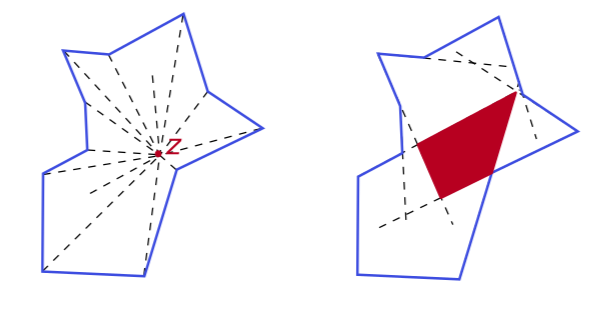
Now a shape is called star-shaped if there’s at least one point inside it from which you can see the entire object. Think of it like a single guard standing inside a room; if there’s a spot where the guard can see every single point on every wall without their view being blocked by another part of the room, then the room is star-shaped. This point is called a kernel point, and the set of all possible points where the guard could stand is called the shape’s visibility kernel. If this kernel is not empty, the shape is star-shaped.
On the left we see an irregular non-convex closed polygon where a kernel point is shown along with the lines that connect it to all other vertices.
On the right we now show its visibility kernel in red, that is the set of all kernel points. Also, it is important to note that the kernel may be computed by simply taking the intersection of all inner half-planes defined by each face, i.e. the half-planes of each face whose normal vector points to the inside of the shape.
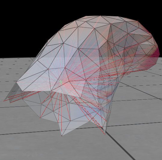
As a 3D example, we shown in the image bellow a 3D mesh of the tip of a thumb, where we can see a green point inside the mesh (a kernel point) from which red lines are drawn to every vertex of the mesh.
3D mesh example showing a kernel point.
Point Sampling
Before we explore the 2 approaches (interior and surface), we first go about finding sample points on the mesh from which to grow the regions. These can be both interior and surface points.
Surface points
To sample points on a 3D surface, several strategies exist, each with distinct advantages. The most common approaches are:
Uniform Sampling: This is the most straightforward method, aiming to distribute points evenly across the surface area of the mesh. It typically works by selecting points randomly, with the probability of selection being proportional to the area of the mesh’s faces. While simple and unbiased, this approach is “blind” to the actual geometry, meaning it can easily miss small but important features like sharp corners or fine details.
Curvature Sampling: This is a more intelligent, adaptive approach that focuses on capturing a shape’s most defining characteristics. The core idea is to sample more densely in regions of high geometric complexity. These areas, often called “interest points,” are identified by their high curvature values, such as Gaussian curvature (\(\kappa_G\)) or mean curvature (\(\kappa_H\)). By prioritizing these salient features (corners, edges, and sharp curves), this method produces a highly descriptive set of sample points that is ideal for creating robust shape descriptors for matching and analysis.
Farthest-Point Sampling (FPS): This iterative algorithm is designed to produce a set of sample points that are maximally spread out across the entire surface. The process is as follows:
A single starting point is chosen randomly.
The next point selected is the one on the mesh that has the greatest geodesic distance (the shortest path along the surface) to the first point.
Each subsequent point is chosen to be the one farthest from the set of all previously selected points.
This process is repeated until the desired number of samples is reached.
In this project we implemented the curvature and FPS methods. However, none of these approaches gave us the desired distribution of points. So we came up with a hybrid approach: Farthest-Point Curvature-Informed sampling (FPCIS) . It aims to achieve a balance between two competing goals:
Coverage: The sampled points should be spread out evenly across the entire surface, avoiding large unsampled gaps. This is the goal of the standard Farthest Point Sampling (FPS) algorithm.
Feature-Awareness: The sampled points should be located at or near geometrically significant features, such as sharp edges, corners, or deep indentations. This is where curvature comes into play.
We start by selecting the highest curvature point in the mesh. Then, similar to FPS we compute the geodesic distances from this selected point to all other points using the Dijkstra algorithm over the mesh. However, instead of just taking the farthest point, we first create a pool of the top 30% farthest points, and from this pool we then select the one with highest curvature. The subsequent points are chosen in a similar manner to FPS.
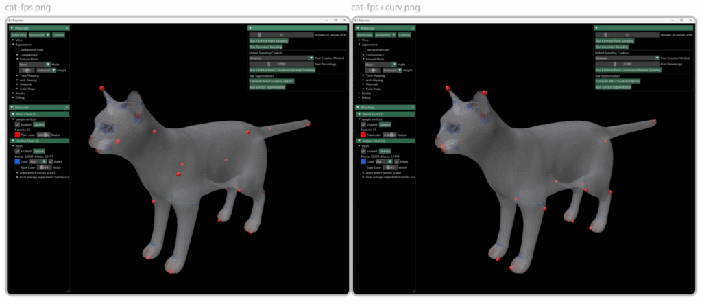
Visualization of surface point sampling methods created using Polyscope.
The image above shows the sampling of 15 points using pure FPS (left) and using the FPCIS (right). we see that although FPS gives a pretty well distributed set of sample points we found that some regions that we deemed important where being left out. For example, when sampling 15 points using FPS on the cat model one of the ears was not being sampled. When using the curvature-informed approach we can see that the important regions are correctly sampled.
Interior points
To achieve a list of points that lie well inside the mesh and have good visibility out to the surface, we cast rays inward from every face and recording where they first hit the opposite side of the mesh. Concretely:
For each triangular face, we compute its centroid.
We flip the standard outward face normal to get an inward direction \(d\).
From each centroid, we cast a ray along \(d\), offset by a tiny \(\epsilon\) so it doesn’t immediately self‐intersect.
We use the Möller–Trumbore algorithm to find the first triangle hit by each ray.
The midpoint between the ray origin and its first intersection point becomes one of our skeletal nodes—a candidate interior sample.
Casting one ray per face can produce thousands of skeletal nodes. We apply two complementary down‐sampling techniques to reduce this to a few dozen well‐distributed guards:
EuclideanFarthest Point Sampling (FPS)
Start from an arbitrary seed node.
Iteratively pick the next node that maximizes the minimum Euclidean distance to all previously selected samples.
This spreads points evenly over the interior “skeleton” of the mesh.
k-Means Clustering
Cluster all the midpoints into k groups via standard k-means in \(\mathbb R^3\).
Use each cluster centroid as a down‐sampled guard point.
This tends to place more guards in densely populated skeleton regions while still covering sparser areas.
Interior Approach
Building upon the interior points sampled earlier, Yu & Li (2011) proposed 2 methods to decompose the mesh into star-shaped pieces: Greedy and Optimal.
1. Greedy Strategy
To achieve this, we solve a fast set-cover heuristic:
Repeatedly pick the guard whose visible-face set covers the most currently uncovered faces, remove those faces, and repeat until every face is covered.
For each guard \(g\), we shoot one ray per face-centroid to decide which faces it can “see.” We store these as sets $$ C_j=\{i: \text{face i is visible from } g_j\}$$
Let \(U = { 0,1,…, |F|−1}\) be the set of all uncovered faces.
Repeat the following steps until \(U\) is empty:
For each guard j, compute the number of new faces it would cover: $$ s_j = | C_j \cap U | $$
Pick the guard j with the largest \(s_j\).
Record one star-patch of size \(s_j\).
Remove those faces: \(U = U \backslash C_j\).
Output: Get a list of guard indices (= number of star-shaped pieces) that covers the entire mesh.
2. Optimal Strategy
To get the fewest possible star-pieces from the pre-determined finite set of candidate guards, we cast the problem exactly as a minimum set-cover integer program:
Decision variables: Introduce binary \(x_j \in \{0,1\}\) for each guard \(g_j\).
Every face i must be covered by at least one selected guard (constraint) and we aim to minimize the total number of guards (thus pieces), hence together we solve:
The overall pipeline of our implementation is as follows:
We build the \(|F| \times L\) visibility matrix in sparse COO format.
We feed it to SciPy’s milp, wrapping the “≥1” rows in a LinearConstraint and all variables as binary in a single Bounds object.
The solver returns the provably optimal set of \(x_j\). The optimization problem can be stated as \(\min \sum_{i=1}^m x_i\) subject to \(x_i=0,1\) and \(\sum_{j\in J(i)} x_j\ge 1, \forall i\in\{1,\dots,n\}\).
Experimental Results
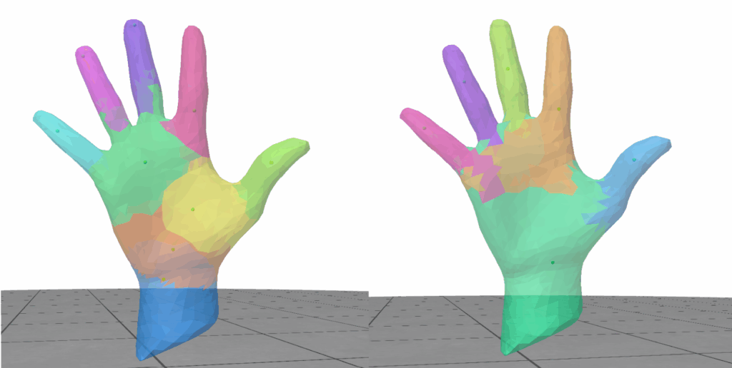
We ran both methods on a human hand mesh with 1515 vertices and 3026 faces. The results are shown below:
Results from Greedy algorithm (left) and Optimal ILP solver (right)
Down-sampling method
Strategy
# of candidate guards
# of star-shaped pieces
Piece connectivity
FPS sampling
Greedy
25
13
No
50
9
Yes
Optimal
25
9
No
50
6
No
K-means clustering
Greedy
25
8
No
50
8
No
Optimal
25
7
No
50
6
No
Some key observations are:
Both interior approaches have no constraints to ensure connectivity among faces of the same guard, hence causing difficulties in closing the mesh of each piece or inaccurate calculation of final connected piece number.
Down-sampling methods: k‐means clustering tends to slightly better distribute guards in high‐density skeleton regions, hence having a smaller gap between greedy and optimal strategy.
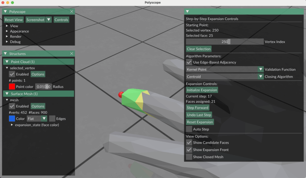
Surface Approach: Surface-Guided Growth with Mesh Closure
One surface-based strategy we explored is a region-growing method guided by local surface connectivity and kernel validation, with explicit mesh closure at each step. The goal is to grow star-shaped regions from sampled points, ensuring at every expansion that the region remains visible from at least one interior point.
This method operates in parallel for each of the N sampled seed points. Each seed initiates its own region and grows iteratively by considering adjacent faces.
Expansion Process
Initialization:
Begin with the seed vertex and its immediate 1-ring neighborhood—i.e., the three faces incident to the sampled point.
Iterative Expansion:
Identify all candidate faces adjacent to the current region (i.e., faces sharing an edge with the region boundary).
Sort candidates by distance to the original seed point.
For each candidate face:
Temporarily add the face to the region.
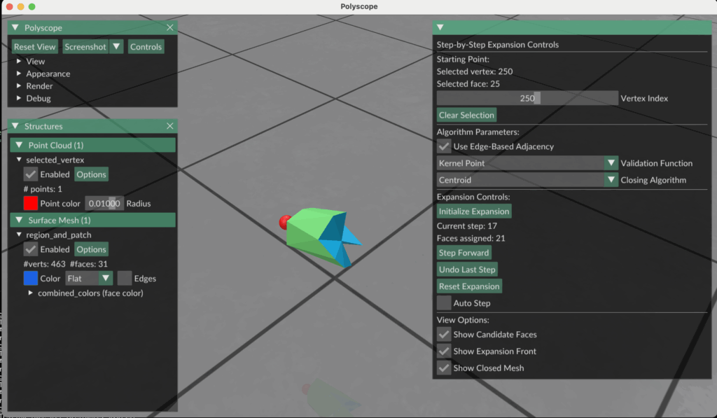
Close the region to form a watertight patch using one of the following mesh-closing strategies:
Centroid Fan – Connect boundary vertices to their centroid to create triangles.
2D Projection + Delaunay – Project the boundary to a plane and apply a Delaunay triangulation.
Run a kernel visibility check: determine if there exists a point (the kernel) from which all faces in the current region + patch are visible.
If the check passes, accept the face and continue.
If not, discard the face and try the next closest candidate.
If no valid candidates remain, finalize the region and stop its expansion.
Results and Conclusions
The kernel check was not robust enough—some regions were allowed to grow into areas that clearly violated visibility constraints.
Region boundaries could expand too aggressively, reaching parts of the mesh that shouldn’t logically belong to the same star-shaped segment.
Small errors in patch construction led to instability in the visibility test, particularly for thin or highly curved regions.
As such, the final segmentations were often overextended or incoherent, failing to produce clean, usable star regions. Despite these issues, this approach remains a useful prototype for purely surface-based decomposition, offering a baseline for future improvements in kernel validation and mesh closure strategies.
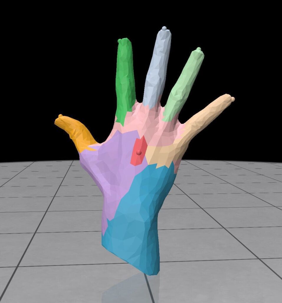
Expansion with the acquired region at the step.
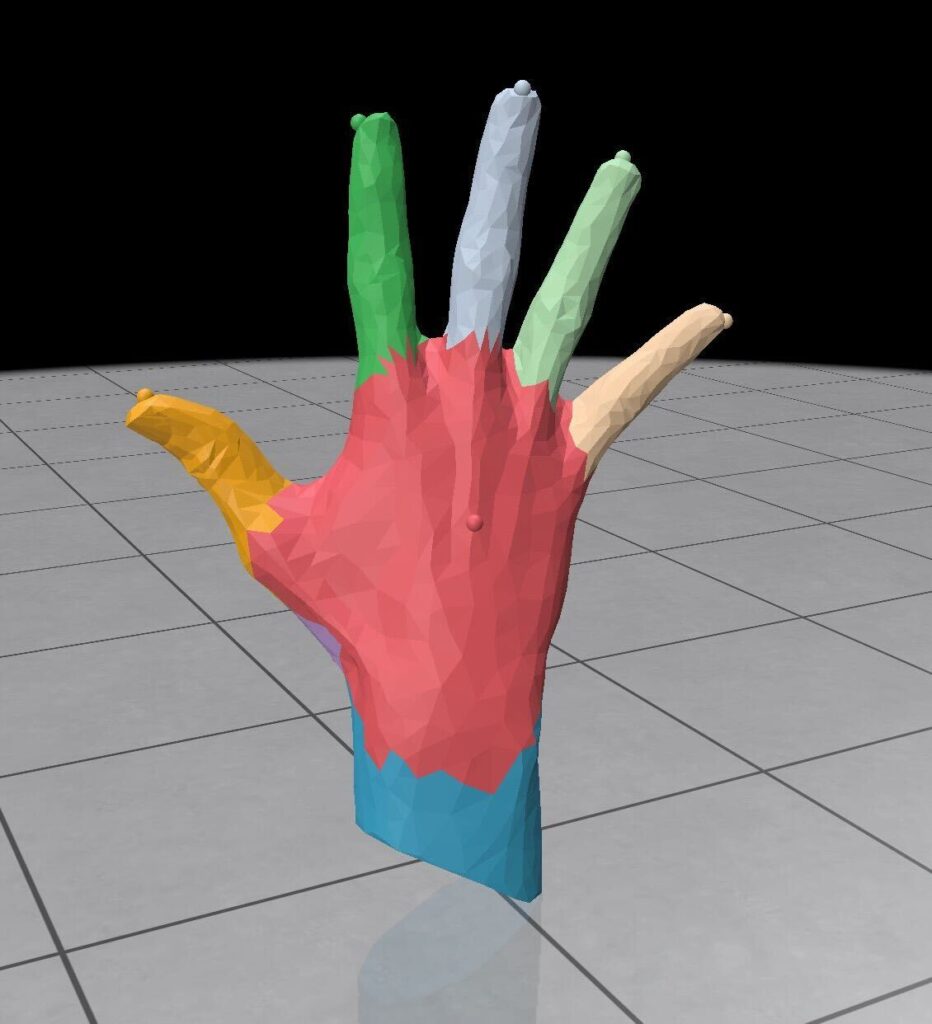
Expansion step showing mesh and its closing patch.
References
Steffen Hinderink, Hendrik Brückler, and Marcel Campen. (2024). Bijective Volumetric Mapping via Star Decomposition. ACM Trans. Graph. 43, 6, Article 168 (December 2024), 11 pages. https://doi.org/10.1145/3687950
Project Mentors: Sainan Liu, Ilke Demir and Alexey Soupikov
Volunteer Assistant: Vivien van Veldhuizen
Introduction
What is Gaussian Splatting?
3D Gaussian Splatting (3DGS) is a new technique for scene reconstruction and rendering. Introduced in 2023 (Kerbl et al., 2023), it sits in the same family of methods as Neural Radiance Fields (NeRFs) and point clouds, but introduces key innovations that make it both faster and more visually compelling.
To better understand where Gaussian Splatting fits in, let’s take a quick look at how traditional 3D rendering works. For decades, the standard approach to building 3D scenes has relied on mesh modelling — a representation built from vertices, edges, and faces that form geometric surfaces. These meshes are incredibly flexible and are used in everything from video games to 3D printing. However, mesh-based pipelines can be computationally intensive to render and are not ideal for reconstructing scenes directly from real-world imagery, especially when the geometry is complex or partially occluded.
This is where Gaussian Splatting comes in. Instead of relying on rigid mesh geometry, it represents scenes using a cloud of 3D Gaussians — small, volumetric blobs that each carry position, color, opacity, and orientation. These Gaussians are optimized directly from multiple 2D images and then splatted (projected) onto the image plane during rendering. The result is a smooth, continuous representation that can be rendered extremely fast and often looks more natural than mesh reconstructions. It’s particularly well-suited for real-time applications, free-viewpoint rendering, and artistic manipulation, which makes it a perfect match for style transfer, as we’ll see next.
What is Style Transfer?
Figure 1: 2D Style Transfer via Neural Algorithm (Gatys et al., 2015)
Style transfer is a technique in computer vision and graphics that allows us to reimagine a given image (or in our case, a 3D scene) by applying the visual characteristics of another image, known as the style reference. In its most familiar form, style transfer is used to turn photos into “paintings” in the style of artists like Van Gogh or Picasso, as seen in Figure 1. This is typically done by separating the content and style components of an image using deep neural networks, and then recombining them into a new, stylized output.
Traditionally, style transfer has been limited to 2D images, where convolutional neural networks (CNNs) learn to encode texture, color, and brushstroke patterns. But extending this to 3D representations — especially ones that support free-viewpoint rendering — has remained a challenge. How do you preserve spatial consistency, depth, and lighting, while also injecting artistic style?
This is exactly the challenge we’re exploring in our project: applying style transfer to 3D scenes represented with Gaussian Splatting. Unlike meshes or voxels, Gaussians are inherently fuzzy, continuous, and rich in appearance attributes, making them a surprisingly flexible canvas for artistic manipulation. By modifying their colors, densities, or even shapes based on style references, we aim for new forms of stylized 3D content — imagine dreamy impressionist cityscapes or comic-book-like architectural walkthroughs. While achieving consistent and efficient rendering in all cases remains an open challenge, Gaussian Splatting offers a promising foundation for exploring artistic control in 3D.
We present a brief comparison of StyleGaussian and ABC-GS baselines, aiming to extend to style transfer for dynamic patterns, 4D scenes, and localized regions of 3DGS.
Style Gaussian Method
The StyleGaussian pipeline (Liu et al., 2024) achieves stylized rendering of Gaussians with real-time rendering and multi-view consistency through three key steps for style transfer: embedding, transfer, and decoding.
Step 1: Feature Embedding Given a Gaussian Splat and camera positions, the first stage of stylization is embedding deep visual features into the Gaussians. To do this, StyleGaussian uses VGG, a classical CNN architecture trained for image classification. Specifically, features are extracted from the ReLU3_1 layer, which captures mid-level textures like edges and contours that are useful for stylization. These are called VGG features, and they act like high-level visual descriptors of the content of an image. However, VGG features are high-dimensional (256 channels or more), and trying to render them directly through Gaussian Splatting might overwhelm the GPU.
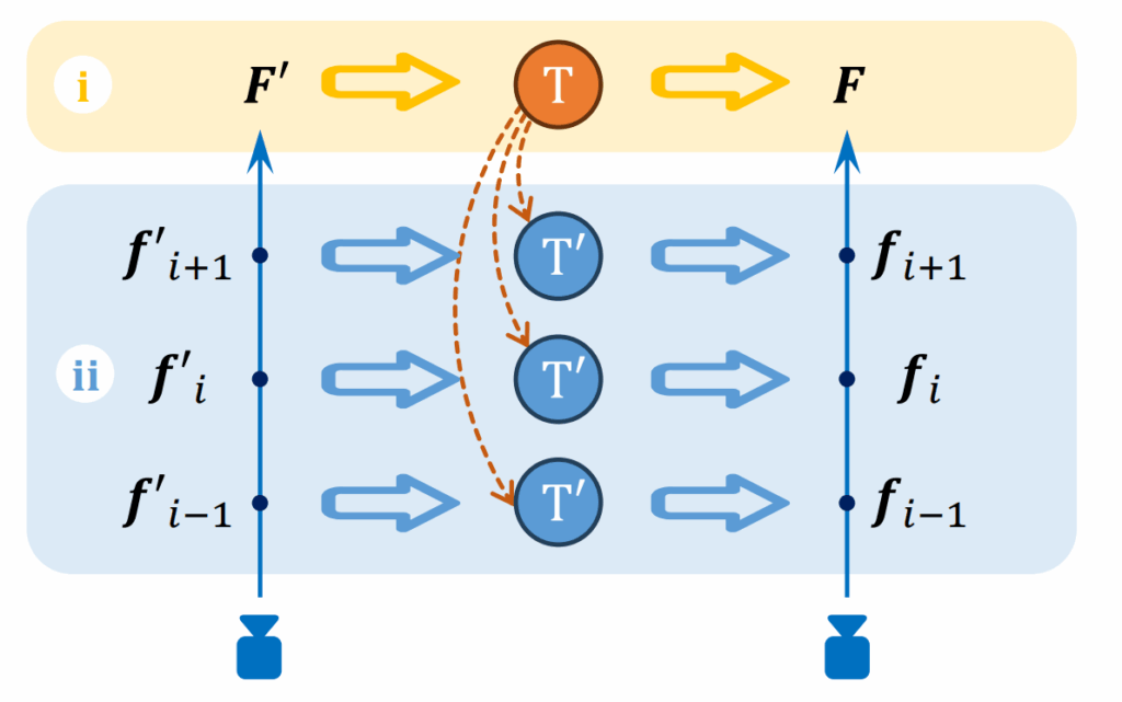
Figure 2: Transformations for Efficient Feature Embedding (Liu et al., 2024)
To solve this, StyleGaussian uses a clever two-step trick illustrated in Figure 2. Instead of rendering all 256 dimensions at once, the program first renders a compressed 32-dimensional feature representation, shown as F’ in the diagram. Then, it applies an affine transformation T to map those low-dimensional features back up to full VGG features F. This transformation can either be done at the level of pixels (i) or at the level of individual Gaussians (ii) — in either case, we recover high-quality feature embeddings for each Gaussian using much less memory.
During training, the system aims to minimize the difference between predicted and true VGG features, so that each Gaussian carries a compact and style-aware feature representation, ready for stylization in the next step.
Step 2: Style Transfer With VGG features embedded, the next step is to apply the style reference. This is done using a fast, training-free method called AdaIN (Adaptive Instance Normalization). AdaIN works by shifting the mean and variance of the feature vectors for each Gaussian so that they match those of the reference image, “repainting” the features without changing their structure. Since this step is training-free, StyleGaussian can apply any new style in real time.
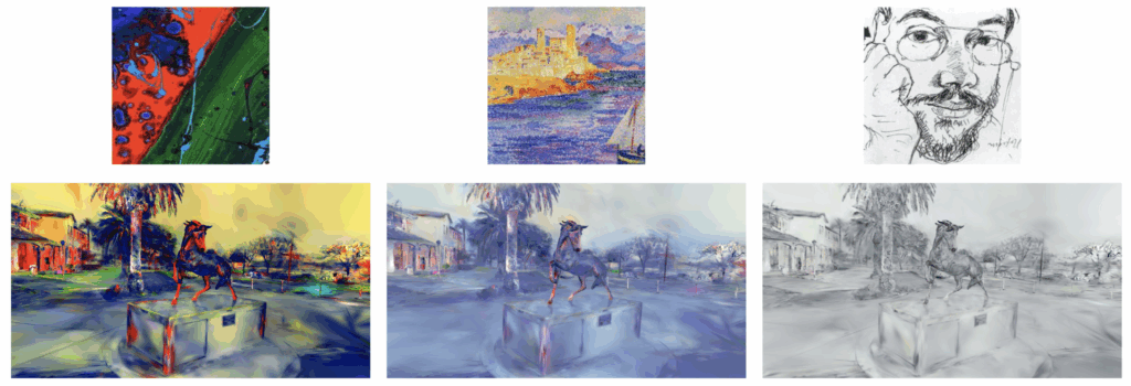
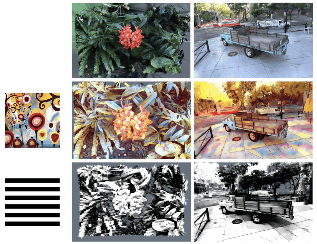
Figure 3: Sample Style Transfer (style references provided by StyleGaussian)
Step 3: RGB Decoding After the style is applied, each Gaussian now carries a modified feature vector — a set of abstract values the neural network uses to describe patterns like brightness, curvature, textures, etc. To render the image, this feature vector needs to be converted into RGB colors for each Gaussian. StyleGaussian does this via a 3D CNN that operates across neighboring Gaussians. This network is trained using a small subset of the style reference images. By comparing a rendered view of the style-transfer to the reference, the network learns how to color the entire scene in a way that reflects the chosen artistic style.
ABC-GS Method
While StyleGaussian offers impressive real-time stylization using feature embeddings and AdaIN, it has a major limitation: it treats the entire scene as a single unit. That means the style is applied uniformly across the whole 3D reconstruction, with no understanding of different objects or regions within the scene.
This is where ABC-GS (Alignment-Based Controllable Style Transfer for 3D Gaussian Splatting) brings something new to the table.
Rather than applying style globally, ABC-GS (Liu et al., 2025) introduces controllability and region-specific styling, enabling three distinct modes of operation:
Single-image style transfer: Apply the visual style of a single image uniformly across the 3D scene, similar to traditional style transfer.
Compositional style transfer: Blend multiple style images, each assigned to a different region of the scene. These regions are defined by manual or automatic masks on the content images (e.g., using SAM or custom annotation). For example, one style image can be applied to the sky, another to buildings, and a third to the ground — each with independent control.
Semantic-aware style transfer: Use a single style image that contains multiple internal styles or textures. You extract distinct regions from this style image (e.g., clouds, grass, brushstrokes) and assign them to matching parts of the scene (e.g., sky, ground) via semantic masks of the content. These masks can be generated automatically (with SAM) or refined manually. This allows for highly detailed region-to-region alignment even within one image.
Figure 4: ABC-GS Single Image Style Transfer
The Two-Stage Stylization Pipeline
ABC-GS achieves stylization using a two-stage pipeline:
Stage 1: Controllable Matching Stage (used in modes 2 and 3 only) In compositional and semantic-aware modes, this stage prepares the scene for region-based style transfer. It includes:
Mask projection: Content and style masks are projected onto the 3D Gaussians.
Style isolation: Each region of the style image is isolated to avoid texture leakage.
Color matching: A linear color transform aligns the base colors of each content region with its assigned style region.
This stage is not used in the single-image mode, since the entire scene is styled uniformly without regional separation.
Stage 2: Stylization Stage (used in all modes) In all three modes, the scene undergoes optimization using the FAST loss (Feature Alignment Style Transfer). This loss improves upon older methods like NNFM by aligning entire distributions of features between the style image and the rendered scene. It captures global patterns such as brushstroke directions, color palette balance, and texture consistency – even in single-image style transfer, FAST consistently yields more coherent and faithful results.
To preserve geometry and content, the stylization is further regularized with:
Content loss: Retains original image features.
Depth loss: Maintains 3D structure.
Regularization terms: Prevent artifacts like over-smoothed or needle-like Gaussians.
Together, these stages make ABC-GS uniquely capable of delivering stylized 3D scenes that are both artistically expressive and structurally accurate — with fine-grained control over what gets stylized and how.
Visual & Quantitative Comparison
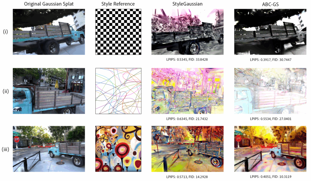
Figure 5 illustrates style transfer applied to a truck composed of approximately 300k Gaussians by StyleGaussian (left) and ABC-GS (right). In choosing simple patterns like a checkerboard or curved lines, we hope to highlight how each method handles the key challenges of 3D style transfer, such as alignment with underlying geometry, multi-view consistency, and accurate pattern representation.
To evaluate these differences from a quantitative angle, Fréchet Inception Distance (FID) and Learned Perceptual Image Patch Similarity (LPIPS) metrics were used.
FID measures the distance between the feature distributions of two images sets, with lower scores indicating greater similarity. This metric is often used in generative adversarial network (GAN) and neural style transfer research to assess how well generated images match a target domain. Meanwhile, LPIPS measures perceptual similarity between image pairs by comparing deep features from a pre-trained network, with lower scores indicating better content preservation.
For our purposes, FID measures style fidelity (how well stylized images match the style reference), with scores generally between 0 and 200, and lower scores indicating strong style similarity. LPIPS measures geometry and content preservation (how well the original scene structure is retained) within a range [0, 1], with lower scores indicating better structural preservation.
Figure 5: Comparison between StyleGaussian and ABC-GS
There is a clear visual improvement in the geometric alignment of patterns in the ABC-GS style transfer, where patterns adhere more cleanly with the object boundaries. In contrast, StyleGaussian shows a more diffuse application, with some color-bleeding and areas with high pattern variance (e.g., the wooden panels on the truck). In terms of LPIPS and FID scores, ABC-GS generally outperforms StyleGaussian, but tends to apply a less stylistically-accurate transfer with regular patterns (i) compared to more “abstract” ones (iii).
This difference in performance may stem from how StyleGaussian and ABC-GS handle feature alignment and geometry preservation. StyleGaussian applies a zero-shot AdaIN shift to all Gaussians, matching only the mean and variance of features; since higher-order structure is ignored, patterns can drift onto the wrong parts of the geometry. In contrast, ABC-GS optimizes the scene via FAST loss, computing a transformation that aligns the entire feature distribution of the rendered scene to that of the style. Meanwhile, content loss keeps the scene recognizable, depth loss maintains 3D geometry, and Gaussian regularization prevents distortions, resulting in better LPIPS and FID scores overall. However, in a case like (ii) where there is a lot of white background, ABC-GS’s competing content, depth, and regularization losses prevent large areas to be overwritten with pure white. Instead, it will try to keep more of the original scene’s detail and contrast, especially around geometry edges, which causes a deviation from the style reference and higher FID score. This interplay between geometry and style preservation is a key tradeoff in style transfer.
Although FID and LPIPS metrics are well-established in 2D image synthesis and style transfer, it is important to recognize potential limitations of applying them directly to 3D style transfer. These metrics operate on individual rendered views, without considering multi-view consistency, depth alignment, or temporal coherence. Future works should aim to better understand these benchmarks for 3D scenes.
Extensions & Experiments
Localized Style Transfer: Unsupervised Structural Decomposition of a LEGO Bulldozer via Gaussian Splat Clustering
We explore a novel technique for structural decomposition of complex 3D objects using the latent feature space of Gaussian Splatting. Rather than relying on pre-defined semantic labels or handcrafted segmentation heuristics, we directly use the parameters of a trained Gaussian Splat model as a feature embedding for clustering.
Motivation
The aim was twofold:
Discovery – to see whether clustering Gaussians reveals structural groupings that are not immediately obvious from the visual appearance.
Applicability – to explore whether these groupings could be useful for style transfer workflows, where distinct regions of a 3D object might be stylized differently based on structural identity.
Method
We trained a Gaussian Splatting model on a multi-view dataset of a LEGO bulldozer. The model was optimized to reconstruct the object from multiple angles, producing a 3D representation composed of thousands of oriented Gaussians.
From this representation, we extracted the following features per Gaussian:
3D Position(x, y, z) (weighted for stronger spatial influence)
Color(r, g, b)
Scale(scale_0, scale_1, scale_2) (downweighted to avoid overemphasis)
Opacity(if available)
Normal Vector(nx, ny, nz)(surface orientation)
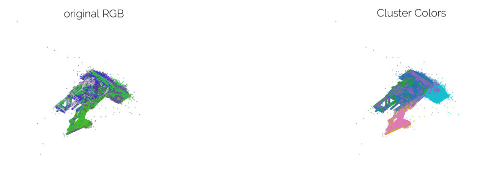
These features were concatenated into a single vector per Gaussian, weighted appropriately, and standardized. We applied KMeans clustering to segment the Gaussian set into six groups.
Results
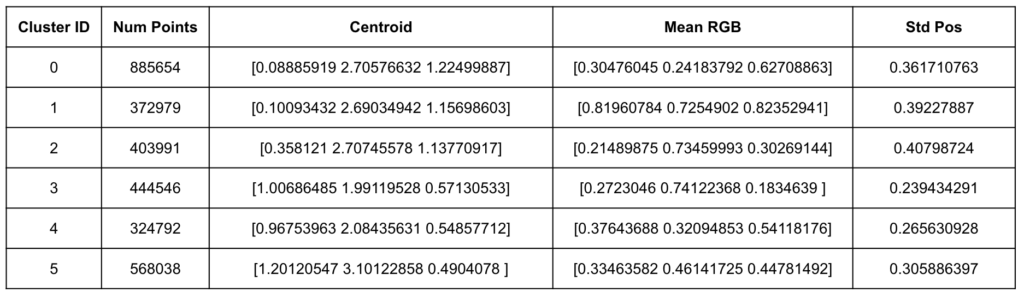
The clustering revealed six distinct regions within the bulldozer’s Gaussian representation, each with unique spatial, chromatic, and geometric signatures.
Figure 6: Statistics for 6 Clusters
Figure 7: Visualization of KMeans groupings
Conclusion
The clustering was able to segment the bulldozer into regions that loosely align with intuitive sub-parts (e.g., the bucket, cabin, and rear assembly), but also revealed less obvious groupings—particularly in areas with subtle differences in surface orientation and scale that are hard to distinguish visually. This suggests that Gaussian-parameter-based clustering could serve as a powerful tool for automated part segmentation without requiring labeled data.
Future Work
Cluster Refinement – Experiment with different weighting schemes and feature subsets (e.g., excluding normals or opacity) to evaluate their effect on segmentation granularity.
Hierarchical Clustering – Apply multi-level clustering to capture both coarse and fine structural groupings.
Style Transfer Applications – Use cluster assignments to drive localized style transformations, such as recoloring or geometric exaggeration, to test their value in content creation workflows.
Cross-Object Comparison – Compare clustering patterns across different models to see if similar structural motifs emerge.
Dynamic Texture Style Transfer
Next, given StyleGaussian’s ability to apply new style references at runtime, a natural extension is style transfer of dynamic patterns. Below are some initial results of this approach, created by cycling through the frames of a gif or video in predetermined time intervals.
There is a key tradeoff between flexibility and quality: while zero-shot transfer enables dynamic patterns, the features are relatively muddled, making it difficult to project detailed media. Meanwhile, in the case of ABC-GS, this improved stylization is a result of optimization, which cannot occur at runtime as with StyleGaussian, making it difficult to render dynamic patterns.
Dynamic Scene Style Transfer
So far we’ve shown how incredibly powerful 3D Gaussian Splatting (3DGS) is for generating 3D static scene representations with remarkable detail and efficiency. The parallel to the dawn of photography is a compelling one: just as early cameras first captured the world on a static 2D canvas, 3DGS excels at creating photorealistic representations of real world scenes on a static 3D canvas. A logical next step is to leverage this technology to capture dynamic scenes.
Videos represent dynamic 2D scenes by capturing a series of static images that, when shown in rapid succession, let us perceive subtle changes as motion. In a similar fashion, one may attempt to capture dynamic 3D scenes as a sequence of static 3D scene representations. However, the curse of dimensionality plagues any naive approach to bring this idea to reality.
Lessons from Video Compression
In the digital age of motion picture, storing a video naively as a sequence of individual images (imitating a physical film strip) is possible but hugely inefficient. A digital image is nothing more than a 2D grid of small elements called pixels. In most image formats, each pixel usually stores about 3 bytes of color data, and a good quality Full HD image contains around 1920 x 1080 ≈ 2 million pixels. This amounts to around 6 million bytes (6 MB) of memory needed to store a single uncompressed Full HD image. Now, a reasonably good video should capture 1 second of a dynamic scene using 24 individual images (24 fps), which yields 144 MB of data to capture just a single second of uncompressed video (using uncompressed images). This means that a quick 30-second video would require a whopping 5 GB of memory.
So although possible, this naive approach to capturing dynamic 2D scenes quickly becomes impractical. To address this problem, researchers and engineers developed compression algorithms for both images and videos in an attempt to reduce memory requirements. The JPEG image format, for example, achieves an average of 10:1 compression ratio, shrinking a Full HD image to only 0.6 MB (600 KB) of storage. However, even if we store a 30-second video as a sequence of compressed JPEG frames, we would still be looking at a 500 MB video file.
The JPEG format compresses images by removing unnecessary and redundant information on the spatial domain, identifying patterns in different parts of the image. Following this same principle, video formats like MP4 identify patterns in the time domain and use them to construct a motion vector field to shift parts of the image from one frame to another. By storing only what changes, these video formats often achieve around 100:1 compression — depending on the contents of the scene — which takes our original 30-second 5 GB video to only 50 MB.
We will now see how this problem of scalability gets even worse when dealing with 3D Gaussian Splatting scenes.
The Curse of Dimensionality
Previously, we have discussed that while 2D grids are made up of pixels storing 3 bytes of color information, 3DGS Gaussians store position, orientation, scale, opacity, and color data. Thus, it is important to note that an image represents a scene from a single viewpoint, so its lighting information is static and can be easily stored using simple RGB colors. In contrast, since GS must represent a 3D scene from various viewpoints, we must have a way to store this dynamic lighting and change Gaussians’ colors depending on where the scene is viewed from. To achieve this, a technique called Spherical Harmonics is used to encode both color and lighting information for each Gaussian.
To store this information we need:
3 floats for position,
3 floats for scale,
4 floats for orientation (using quaternions),
1 float for opacity,
16 floats for color/lighting (using spherical harmonics*).
Using single-precision floats, that is 236 bytes per Gaussian. In a crude comparison, we can see that the building blocks of a 3DGS scene representation must store 78x more data than a pixel in a 2D image. While the next section shows that good 3DGS scenes require much fewer Gaussians than a good image requires pixels, moving to the 3rd dimension already poses a significant memory challenge.
For example, Figure 8 contains around 200.000 Gaussians, which amounts to about 23 MB of data for a single static scene.
Figure 8: Lego Bulldozer with 200k Gaussians, generated with PostShot
If we were to follow the same naive idea for 2D videos and store a full static scene for each frame of a dynamic scene, we would need 24 static 3DGSs to represent 1 second of the dynamic scene (at 24 FPS), which would require 550 MB. A 30-second clip would then require a whopping 15 GB of storage. For more complex or detailed scenes, this problem only gets worse. And that’s just storage; generating and rendering all of this information would require a lot of computation and memory bandwidth, especially if we aim for real-time performance.
One notable approach to this problem was presented by Luiten et al. (2023), where the authors take a canonical set of Gaussians and keep intrinsic properties like color, size and opacity constant in time, storing only the position and orientation of Gaussians at each timestep. While less data is needed for each frame, this approach still scales linearly with frame count.
A Solution: Learn How the Scene Changes
So, instead of representing dynamic scenes as sequences of static 3DGS frames, a compelling research direction is to employ a strategy similar to video compression algorithms: focus on encoding how the scene changes between frames.
This is the idea behind 4D Gaussian Splatting for Real-Time Dynamic Scene Rendering (Wu et al., 2024). Their solution comes in the form of a Gaussian Deformation Field Network, a compact neural network that implicitly learns the function that dictates motion for the entire scene. This improves scalability, as the memory footprint depends mainly on the network’s size rather than video length.
Instead of redundantly storing scene information, 4DGS establishes a single canonical set of 3D Gaussians, denoted by \( \mathscr{G} \), that serves as the master model for the scene’s geometry. From there, the Gaussian Deformation Field Network \( \mathscr{F}\) learns the temporal evolution of Gaussians. For each timestamp \(t\), the network predicts the deformation \(\Delta \mathscr{G}\) for the entire set of canonical Gaussians. The final state of the scene for that frame, \(\mathscr{G}’\), is then computed by applying the learned transformation:
The network’s encoder is designed with separate heads to predict the components of this transformation: a change in position (\(\Delta \mathscr {X}\)), orientation (\(\Delta r\)), and scale (\(\Delta s\)).
By encoding a scene as fixed geometry (the canonical Gaussian set) plus a learned function of its dynamics, 4DGS offers an efficient and compact model of the dynamic 3D world. Additionally, because the model is a true 4D representation, it enables rendering the dynamic scene from any novel viewpoint in real-time, thereby transforming a simple recording into a fully immersive and interactive experience.
The output is a canonical Gaussian Splatting scene stored as a .ply file together with a set of .pth files (the standard PyTorch model files) that encode the Gaussian Deformation Field Network. From there, the scene may be rendered from any viewpoint at any timestamp of the video.
To demonstrate, we use a scene from the HyperNerf dataset. Figure 9 compares the original video (left), the resulting trained-view 4DGS (center), and the resulting test-view 4DGS (right). The right video is rendered from a different viewpoint and is used to verify that the GS indeed generalized the scene geometry in 3D space.
Figure 9: Broom views from 4DGS
The 4DGS pipeline
Before explaining the 4DGS pipeline, we must first understand its input. We aim to generate a 4D scene — that is a 3D scene that changes over time (+1D). This requires a set of videos that capture the same scene simultaneously. In synthetic datasets, researchers use multiple cameras (e.g., 27 cameras in the Panoptic dataset) to film from multiple viewpoints at the same time. However, in real world setups, this is impractical, and usually a stereo setup (i.e. 2 cameras) is more common, as in the HyperNerf dataset.
With the input defined, the pipeline can be split into 3 main steps:
Initialization: Before anything can move, the model needs a 3D “puppet” to animate. The quality of this initial puppet depends heavily on the camera setup used to film the video.
Case A: The ideal multi-camera setup
Scenario: This applies to lab-grade datasets like the Panoptic Studio dataset, which uses a dome of many cameras (e.g., 27) all recording simultaneously.
Process: The model looks at the images from all cameras at the very first moment in time (t=0). Because it has so many different viewpoints of the scene frozen in that instant, it can use Structure-from-Motion (SfM) to create a highly accurate and dense 3D point cloud.
Result: This point cloud is turned into a high-fidelity canonical set of Gaussians that perfectly represents the scene at the start of the video. It’s a clean, sharp, and well-defined starting point.
Case B: The Challenging real-world scenario
Scenario: This applies to more common videos filmed with only one or two cameras, like those in the HyperNeRF dataset.
Process: With too few viewpoints at any single moment, SfM needs the camera to move over time to build a 3D model. Therefore, the algorithm must analyze a collection of frames (e.g., 200 random frames) from the video.
Result: The static background is reconstructed well, but the moving objects are represented by a more scattered, averaged point cloud. This initial canonical scene doesn’t perfectly match any single frame but instead captures the general space the object moved through. This makes the network’s job much harder.
Static Warm-up: With the initial puppet created, the model spends a “warm-up” period (the first 3,000 iterations in the paper’s experiments) optimizing it as if it were a static, unmoving scene. This step is crucial in both cases. For the multi-camera setup, it fine-tunes an already great model. For the single-camera setup, it’s even more important, as it helps the network pull the averaged points into a more coherent shape before it tries to learn any complex motion.
Dynamic Training: Now for the main step, the model goes through the video frame by frame and trains the Gaussian Deformation Field Network.
Pick a Frame: The training process selects a specific frame (a timestamp, t) from the video.
Ask the Network: It feeds the canonical set of Gaussians \(\mathscr G\) and the timestamp \(t\) into the deformation network \(\mathscr F\).
Predict the motion: The network predicts the necessary transformations \(\Delta \mathscr G\) for every single Gaussian to move them from their canonical starting position to where they should be at a timestamp t. This includes changes in position, orientation and scale.
Apply the motion: The predicted transformations are applied to the canonical Gaussians to create a new set of deformed Gaussians \(\mathscr G’\) for that specific frame.
Render the image: The model then renders the ‘splats’ the deformed Gaussians onto an image, creating a synthetic view of what the scene should look like.
Compare with original and calculate error: The rendered image is then compared with the actual video frame from the dataset. The difference between the two is used as the loss, which is calculated as simply the L1 color loss. It basically says how different each pixel of the splatted image is from the original video frame.
Backpropagation: This is the learning step, where the error is sent backward through the network so it can adjust the position, orientation, and scale of the Gaussians to better approximate the scene.
This loop repeats for different frames and different camera views until the network becomes so good at predicting the deformations that it can generate a photorealistic moving sequence from the single canonical set of Gaussians.
4D Stylization
Now that we understand how 4D Gaussian Splatting works, we present here an idea for integrating the StyleGaussian method into the 4DGS pipeline. Unfortunately we were not able to fully implement this idea due to time limitations, however we will explain how and why this idea should work.
The fact that the 4DGS pipeline works by generating a canonical static representation of the scene makes it suitable for integrating with StyleGaussian. We may simply run it on the canonical scene representation that was generated, and the deformation would then move the stylized gaussians to the right places.
One potential problem with this approach, however, is that the canonical scene generated with real-world scenes captured using a stereo camera setup may not correctly represent moving objects on the scene. Due to the lack of images for the initial frame (only 2) when using these datasets, the 4DGS method utilizes random frames from the whole video to obtain the canonical set of Gaussians, which ends up being an average of the scene. Thus, moving objects will not be correctly captured and if we apply a stylization on this averaged scene, it could potentially lead to a less stable or visually inconsistent application of the style on dynamic elements within the final rendered video.
Overall Conclusions & Future Directions
Given the time and resource constraints of our project, we have shown a visual and quantitative comparison of the preservation of pattern features during style transfer with Style Gaussian and ABC-GS. Additionally, using these baselines, we have experimented with some initial results for style transfer with dynamic patterns, proposed a method for combining StyleGaussian with 4DGS, and developed an effective GS clustering strategy that can be used for localized style applications.
Future research might expand on these experiments by:
Exploring better validation metrics for GS scenes that account for 3D components like multi-view consistency
Developing alternatives to random frames for generating canonical set of Gaussians from stereo camera scenes, which will prevent visually inconsistent stylization
Further refining clustering techniques and developing metrics to evaluate the effectiveness of local stylization
Applications of dynamic textures onto individual local GS components via clustering, building on the global transition effect explored previously. This direction could produce interesting “special effects” such as displaying optical illusions or giving a “fire effect” to a 3DGS scene
References
Gatys, L. A., Ecker, A. S., & Bethge, M. (2015, August 26). A neural algorithm of artistic style. arXiv.org. https://arxiv.org/abs/1508.06576
Kerbl, B., Kopanas, G., Leimkuehler, T., & Drettakis, G. (2023). 3D Gaussian Splatting for Real-Time Radiance Field Rendering. ACM Transactions on Graphics, 42(4), 1–14. https://doi.org/10.1145/3592433
Liu, K., Zhan, F., Xu, M., Theobalt, C., Shao, L., & Lu, S. (2024, March 12). StyleGaussian: Instant 3D Style Transfer with Gaussian Splatting. arXiv.org. https://arxiv.org/abs/2403.07807
Liu, W., Liu, Z., Yang, X., Sha, M., & Li, Y. (2025, March 28). ABC-GS: Alignment-Based Controllable Style Transfer for 3D Gaussian splatting. arXiv.org. https://arxiv.org/abs/2503.22218
Luiten, J., Kopanas, G., Leibe, B., & Ramanan, D. (2023, August 18). Dynamic 3D Gaussians: Tracking by persistent dynamic view synthesis. arXiv.org. https://arxiv.org/abs/2308.09713
Wu, G., Yi, T., Fang, J., Xie, L., Zhang, X., Wei, W., Liu, W., Tian, Q., & Wang, X. (2023, October 12). 4D Gaussian Splatting for Real-Time Dynamic Scene rendering. arXiv.org. https://arxiv.org/abs/2310.08528