SGI Mentor: Justin Solomon
SGI Fellows: Shree Singhi, Nhu (Jade) Tran, Haojun Qiu, Eva Kato
Introduction
The heat equation is one of the canonical diffusion PDEs: it models how “heat” (or any diffusive quantity) spreads out over space as time progresses. Mathematically, let \(u(x,t) \in \mathbb{R}_{\geq 0}\) denote the temperature at spatial location \(x \in \mathbb{R}^{d}\) and time \(t \in \mathbb{R}\). The continuous heat equation is given by
where \(\Delta u (x, t) = \sum_{i=1}^{d} \frac{\partial^2 u}{\partial x_i^2}\) is the Laplace operator representing how local temperature gradients drive heat from hotter to colder regions. On a surface mesh, the spatial domain is typically discretized so that the PDE reduces to a system of ODEs in time, which can be integrated using stable and efficient schemes such as backward Euler. Interestingly, in many applications—including geodesic distance computation 1 and optimal transport 2—it is often more useful to work with the logarithm of the heat rather than the heat itself. For example, Varadhan’s formula states that the geodesic distance \(\phi\) between two points \(x\) and \(x^*\) on a curved domain can be recovered from the short-time asymptotics of the heat kernel:
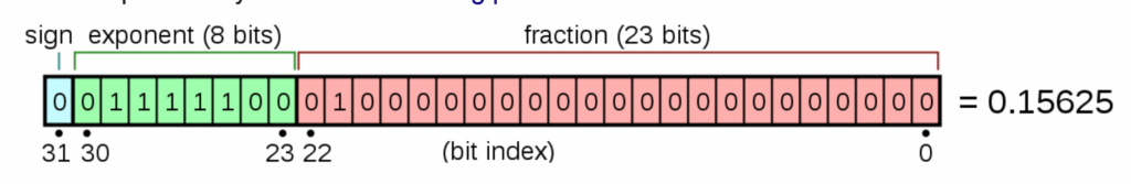
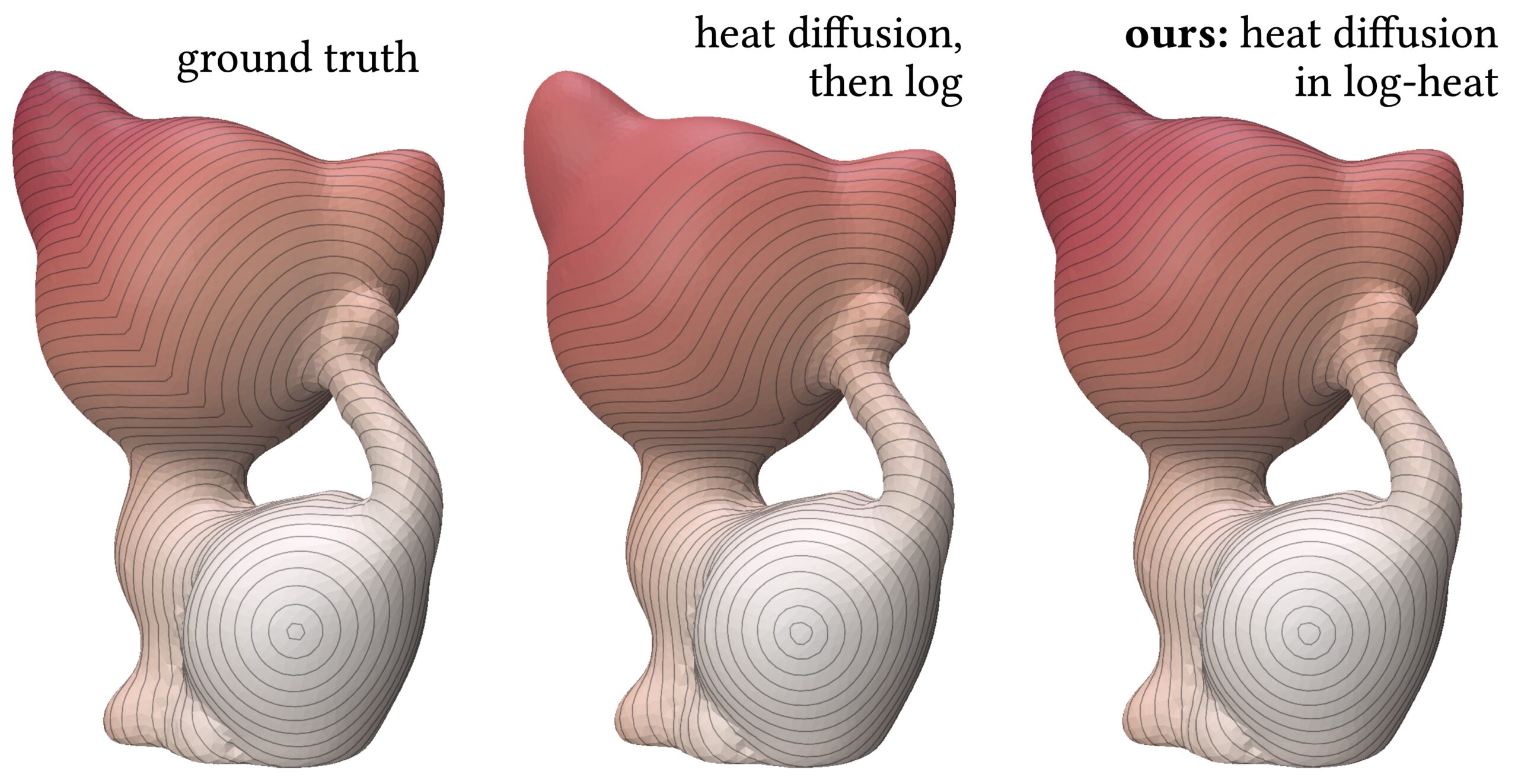
where \(k_{t,x^{*}}(x) = u(x,t)\) is the heat distribution at time \(t\) resulting from an initial Dirac delta at \(x^*\), i.e., \(u(x,0) = \delta(x-x^{*})\). In practice, this leads to a two-step workflow: (1) simulate the heat equation to obtain \(u_t\), and (2) take the logarithm to recover the desired quantity. However, this approach can be numerically unstable in regions where \(u\) is very small: tiny relative errors in \(u\) can be greatly magnified in the log domain. For example, an absolute error of \(10^{-11}\) in \(u\) becomes an error of roughly \(25.33\) in \(\log u\).
A natural idea is therefore to evolve the logarithm of the heat directly. Let \(u>0\) satisfy the heat equation and define \(w = \log u\). One can show that \(w\) obeys the nonlinear PDE 3
This formulation has the appealing property that it avoids taking the logarithm after simulation, thereby reducing the amplification of small relative errors in \(u\) when \(u\) is tiny. However, the price of this reformulation is the additional nonlinear term \(\|\nabla w\|_2^2\), which complicates time integration as each step requires iterative optimization, and introduces a discrepancy with the discretized heat equation. In practice, evaluating \(\|\nabla w\|_2^2\) requires a discrete gradient operator, and the resulting ODE is generally not equivalent to the one obtained by first discretizing the heat equation for \(u\) (which involves only a discrete Laplacian) up to a log transform. This non-equivalence stems from (1) there is a new spatially discretized gradient operator, and (2) the fact that the logarithm is nonlinear and does not commute with discrete differential operators.
Motivated by this discrepancy, we take a different approach that preserves the exact relationship to the standard discretization. We first discretize the heat equation in space, yielding the familiar linear ODE system for \(u\). We then apply the transformation \(w = \log u\) to this discrete system, producing a new ODE for \(w\). Now, by construction, the new ODE is equivalent to the heat ODE up to a log transform of variable. This still allows us to integrate directly in log-space, which allows more accurate and stable computation. We show that this formulation offers improved numerical robustness in regions where \(u\) is very small, and demonstrate its effectiveness in applications such as geodesic distance computation.
| Standard (post-log) | Continuous log-PDE | Proposed discrete-log |
|---|---|---|
| 1. Start with the heat PDE for \(u\). | 1. Start with the log-heat PDE for \(w=\log u\). | 1. Start with the heat PDE for \(u\). |
| 2. Discretize in space \(\Rightarrow\) ODE for \(u\). | 2. Discretize in space for \(\nabla\) and \(\Delta\) \(\Rightarrow\) ODE for \(w\). | 2. Discretize in space \(\Rightarrow\) ODE for \(u\). |
| 3. Time-integrate in \(u\)-space. | 3. Time-integrate in \(w\)-space and output \(w\). | 3. Apply change of variables \(w=\log u\) \(\Rightarrow\) ODE for \(w\). |
| 4. Compute \(w=\log u\) as a post-process. | 4. Time-integrate in \(w\)-space and output \(w\). |
Background
We begin by reviewing how previous approaches are carried out, focusing on the original heat method 1 and the log-heat PDE studied in 3. In particular, we discuss two key stages of the discretization process: (1) spatial discretization, where continuous differential operators such as the Laplacian and gradient are replaced by their discrete counterparts, turning the PDE into an ODE; and (2) time discretization, where a numerical time integrator is applied to solve the resulting ODE. Along the way, we introduce notation that will be used throughout.
Heat Method
Spatial discretization. In the heat method 1, the heat equation is discretized on triangle mesh surfaces by representing the heat values at mesh vertices as a vector \(u \in \mathbb{R}^{|V|}\), where \(|V|\) is the number of vertices. A corresponding discrete Laplace operator is then required to evolve \(u\) in time. Many Laplacian discretizations are possible, each with its own trade-offs 4. The widely used cotangent Laplacian is written in matrix form as \(M^{-1}L\), where \(M, L \in \mathbb{R}^{|V| \times |V|}\). The matrix \(L\) is defined via
where \(i,j\) are vertex indices and \(\alpha_{ij}, \beta_{ij}\) are the two angles opposite the edge \((i,j)\) in the mesh. The mass matrix \(M = \mathrm{diag}(m_1, \dots, m_{|V|})\) is a lumped (diagonal) area matrix, with \(m_i\) denoting the area associated with vertex \(i\). Note that \(L\) has several useful properties: it is sparse, symmetric, and each row sums to zero. This spatial discretization converts the continuous PDE into an ODE for the vector-valued heat function \(u(t)\):
Time discretization and integration. The ODE is typically advanced in time using a fully implicit backward Euler scheme, which is unconditionally stable. For a time step \(\Delta t = t_{n+1} – t_n\), backward Euler yields:
where \(u_n\) is given and we solve for \(u_{n+1}\). Thus, each time stepping requires solving a sparse linear system with system matrix \(M – \Delta t\,L\). Since this matrix remains constant throughout the simulation, it can be factored once (e.g., by Cholesky decomposition) and reused at every iteration, greatly improving efficiency.
Log Heat PDE
Spatial discretization. In prior work 3 on the log-heat PDE, solving this requires discretizing not only the Laplacian term but also the additional nonlinear term \(\|\nabla w\|_2^{2}\). After spatial discretization, the squared gradient norm of a vertex-based vector \(w \in \mathbb{R}^{|V|}\) is computed as
where \(G_{k} \in \mathbb{R}^{|F| \times |V|}\) is the discrete gradient operator on mesh faces for the \(k\)-th coordinate direction, and \(W \in \mathbb{R}^{|V| \times |F|}\) is an averaging operator that maps face values to vertex values. With this discretization, the ODE for \(w(t) \in \mathbb{R}^{|V|}\) becomes
Time discretization and integration. If we apply fully implicit Euler, we would find \(w^{n+1}\) by solving a nonlinear equation. To avoid this large nonlinear solve, prior work 3 splits the problem into two substeps:
- a linear diffusion part: \(\frac{\mathrm{d}w}{\mathrm{d}t} = M^{-1}L\,w\), which is stiff but easy to solve implicitly,
- a nonlinear part: the full equation, which is nonlinear but convex.
This separation lets each component be treated with the method best suited for it: a direct linear solve for the diffusion, and a convex optimization problem for the nonlinear term. Using Strang-Marchuk splitting:
- Half-step diffusion: \((M – \frac{\Delta t}{2} L)\,w^{(1)} = Mw^n\)
- Full-step nonlinear term: Solve a convex optimization problem to find \(w^{(2)}\)
- Half-step diffusion: \((M – \frac{\Delta t}{2} L)\,w^{(3)} = Mw^{(2)}\), and set \(w^{n+1} = w^{(3)}\)
A New ODE in Log-Domain
Let us revisit the spatially discretized heat (or diffusion) equation. For each vertex \(i \in \{1, \dots |V|\}\) on a mesh, its evolution is described by
where \(u\) represents our heat, and \(L\) is the discrete Laplacian operator. A key insight is that the Laplacian term can be rewritten as a sum of local differences between a point and its neighbors:
This shows that the change in \(u_i\) depends on how different it is from its neighbors, weighted by the Laplacian matrix entries. Now, before doing time discretization, we use a change of variable \(w \Leftarrow\log u\), accordingly, \(u = \mathrm{e}^{w}\), to obtain the ODE
which can be rearranged into
In vectorized notation, we construct a matrix \(\tilde{L} \Leftarrow L – \mathrm{diag}(L_{11}, \dots, L_{|V| \,|V|})\), which zeros out the diagonals of \(L\). Then the log heat \(w(t) \in \mathbb{R}^{|V|}\) follows the ODE
and another equivalent way to put it is
This ODE is equivalent to the standard heat ODE up to a log transform of the integrated results, but crucially it avoids the amplification of small relative errors in \(u\) when \(u\) is tiny by integrating directly in log-space.
Numerical Solvers for Our New ODE
Forward (Explicit Euler)
The most straightforward approach uses explicit Euler to update the solution at each time step. The update rule is
While this is efficient and can be solved linearly, it causes instability.
Semi-Implicit
We can discretize with both explicit and implicit parts by decomposing the exponential function as a linear and nonlinear part:
Applying this decomposition yields a linear system for solving \(w_{n+1}\):
This retains efficiency but does not fully address instability issues.
Backward (Convex Optimization)
Solving the backward Euler equation involves finding the vector \(w^{t+1}\) that satisfies
Taking inspiration from prior work 3, we find that relaxing this equality into an inequality leads to a convex constraint on \(w^{t+1}_i\):
It can be shown that minimizing the objective function
with the inequality constraint defined above yields the exact solution to the original equation. We have written a complete proof for this finding here. We implement this constrained optimization problem using the Clarabel solver 6 in CVXPY 7, a Python library for convex optimization problems.
Experiments
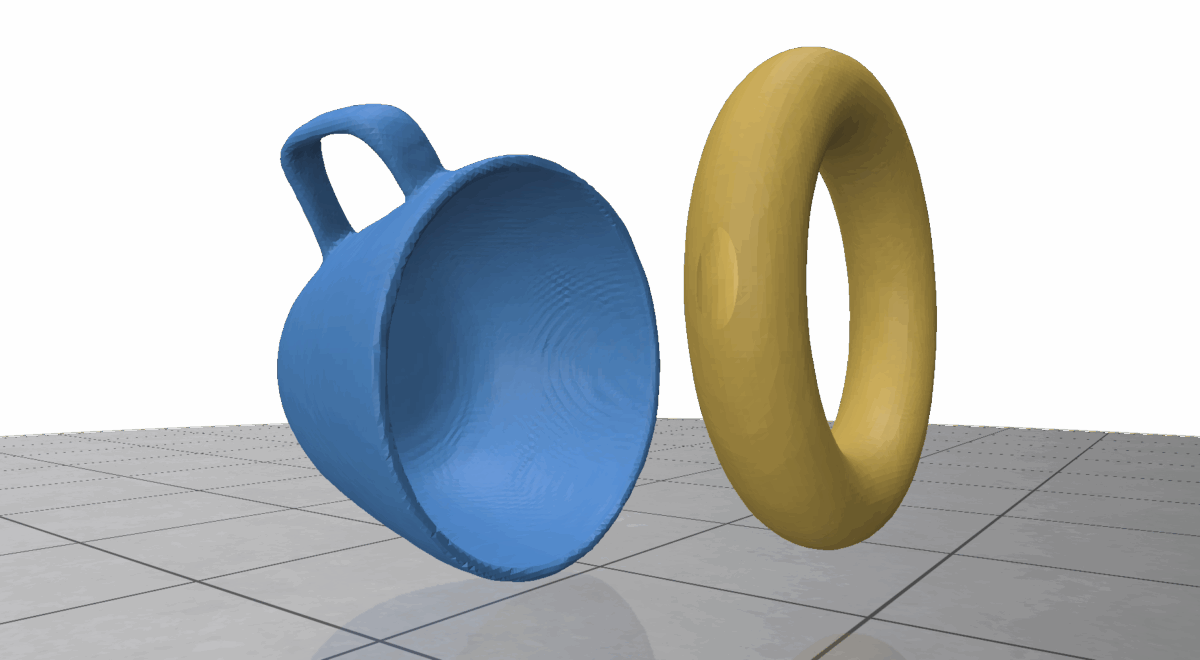
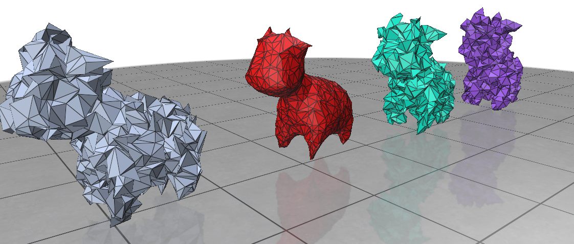
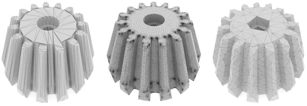
As mentioned earlier, the log heat equation is widely used to efficiently approximate geodesic distances. To evaluate our method, we selected a point on each mesh as a heat source and computed approximate geodesic distances from that point using the log-heat solution with Varadhan’s formula. For comparison, all solvers were applied within the same log-heat framework described in Equation 2 and tested on meshes of varying complexity. As ground truth, we used libigl’s 5 implementation of exact discrete geodesic distances. All experiments used 10 diffusion time-steps equally spaced between \(t = 0\) and \(t = 10^{-2}\). The results are shown in Table 2.
| Mesh | # of verts | Method | Pearson \(r\) ↑ | RMSE ↓ | MAE ↓ |
|---|---|---|---|---|---|
| Lilium | 3389 | HeatBackward | 0.992 | 0.267 | 0.207 |
| LogHeatBackward | 0.653 | 0.510 | 0.385 | ||
| NewLogHeatBackward (ours) | 0.997 | 0.070 | 0.063 | ||
| Cat | 9447 | HeatBackward | 0.991 | 0.063 | 0.043 |
| LogHeatBackward | 0.513 | 0.531 | 0.474 | ||
| NewLogHeatBackward (ours) | 0.998 | 0.150 | 0.140 | ||
| Spot | 11533 | HeatBackward | 0.992 | 0.318 | 0.248 |
| LogHeatBackward | 0.382 | 0.982 | 0.853 | ||
| NewLogHeatBackward (ours) | 0.994 | 0.121 | 0.115 |
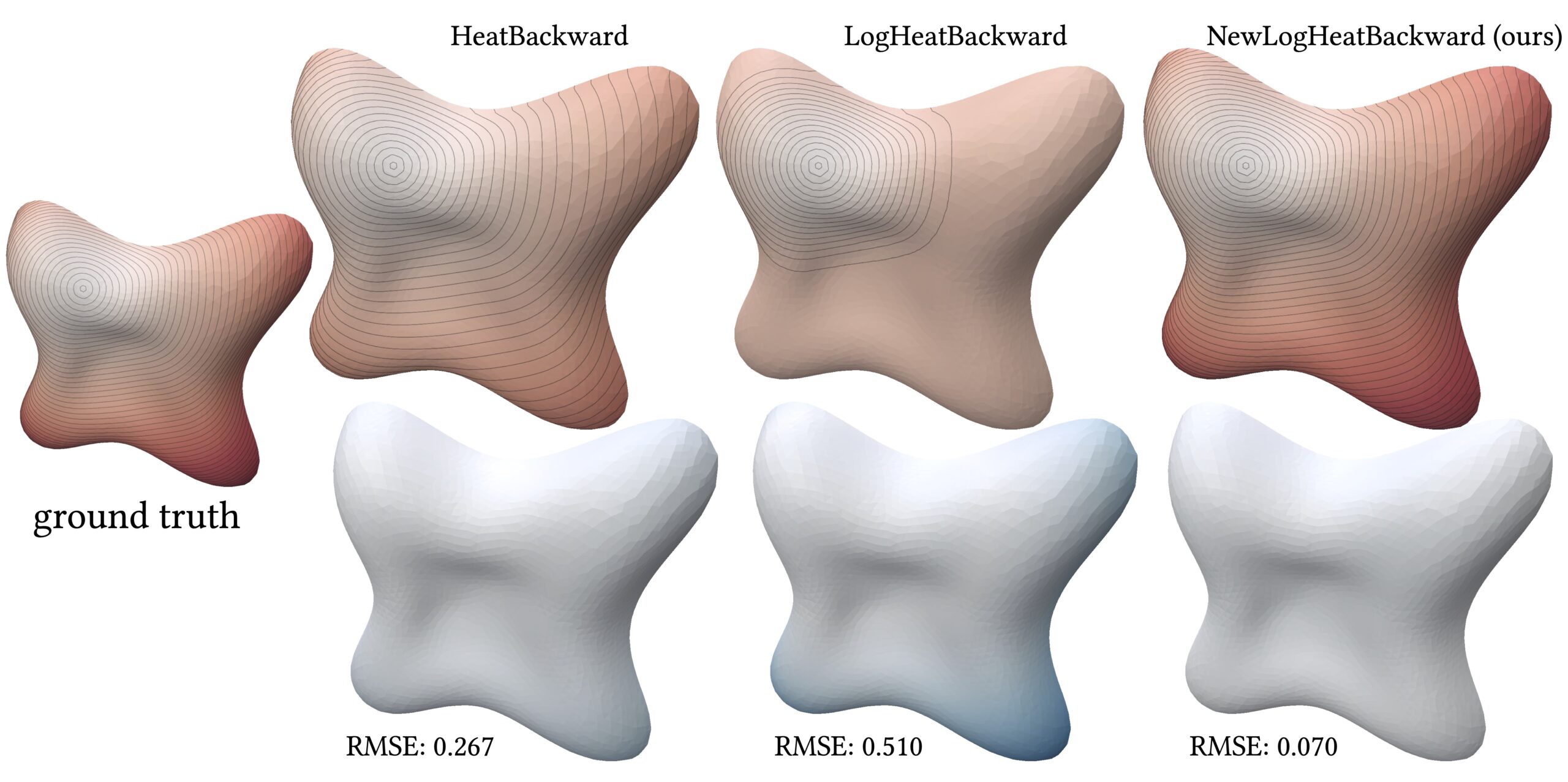
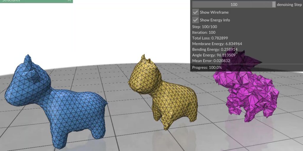
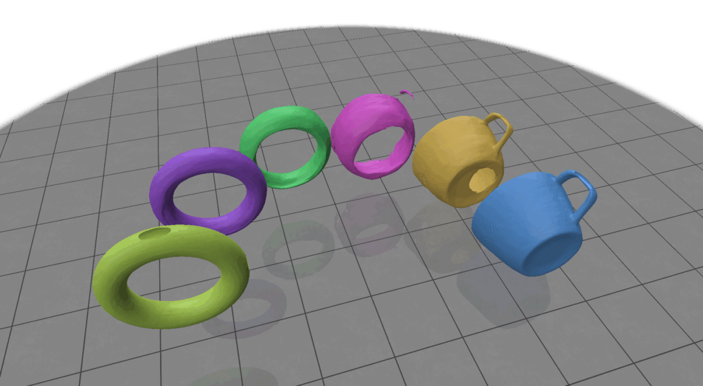
Our method, NewLogHeatBackward, consistently outperforms HeatBackward and LogHeatBackward on all tested meshes, showing the highest correlation with the ground truth while maintaining low RMSE and MAE. This demonstrates that it provides more accurate and reliable approximations of geodesic distances across meshes of different sizes and complexities. While performance can still vary depending on the mesh, NewLogHeatBackward performs especially well on well-behaved meshes, as shown in Figure 2. Figure 3 further illustrates its accuracy by comparing the exact geodesic distances with those computed by each solver. Although the method may slightly overshoot in some cases, it consistently produces results closest to the true geodesic distances.
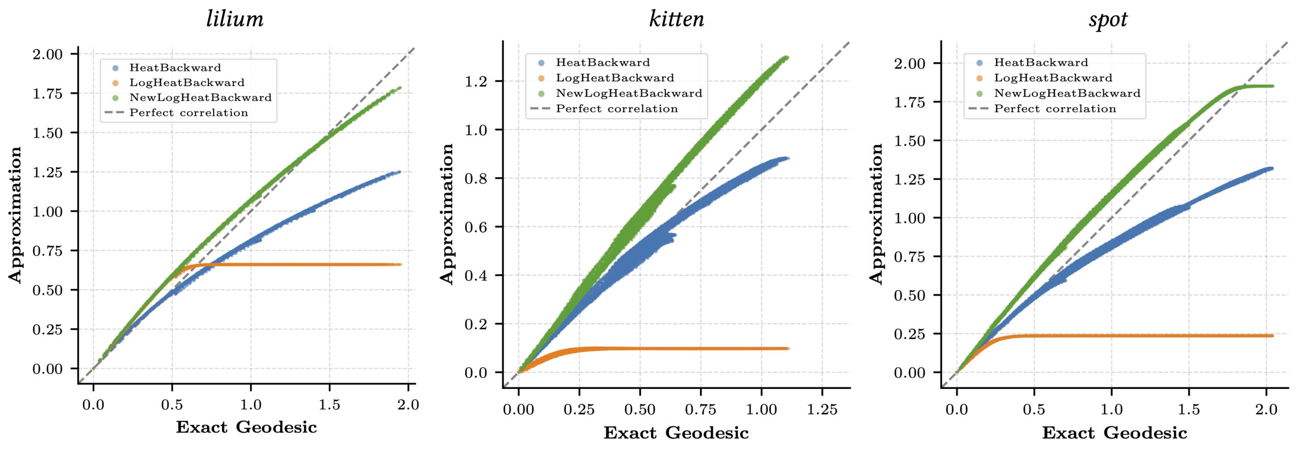
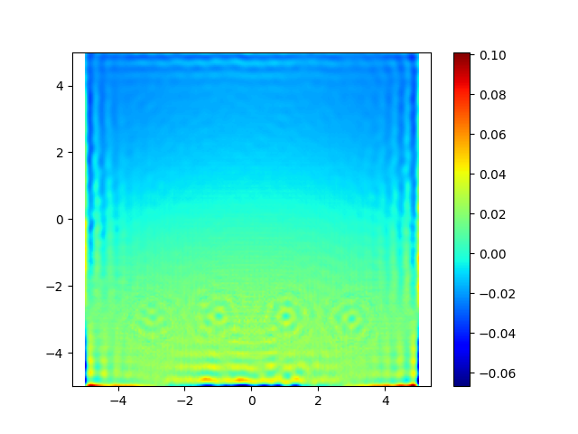
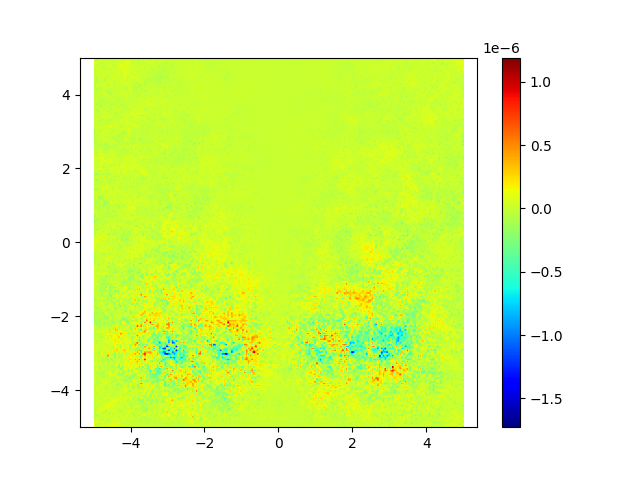
In Figure 1, the flat region for the NewLogHeatBackward Solver probably indicates regions of numerical overflow/underflow, since the log of tiny heat values is going to be incredibly negative. Through our experimentation we observed that the solver for this our formulated PDE outperforms others mostly in cases where the diffusion time-step is extremely small.