One will probably ask “what is even discrete morse theory?”
A good question. But a better question is, “what is even morse theory?”
A Detour to Morse Theory
It would be a sin to not include this picture of a torus on any text for an introduction to Morse Theory.
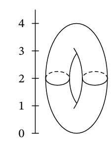
Consider a height function \(f\) defined on this torus \(T\). Let \(M_z = \{x\in T | f(x)\le z\}\), i.e., a slice of the torus below level \(z\).
Morse theory says critical points of \(f\) can tell us something about the topology of the shape. The critical points can be determined by recalling from calculus that those points correspond to the points where the partial derivatives all equal zero. Then, the four critical points on the torus at heights 0, 1, 3, and 4 can be identified, each of which correspond to topological changes in the sublevel sets (\(M_z\)) of the function. In particular, imagine a sequence of sublevel sets \(M_z\) with ever increasing \(z\) values. Notice that each time we pass through a critical point, there is an important topological change in the sublevel sets.
- At height 0, everything starts with a point
- At height 1, a 1-handle is attached
- At height 3, another 1-handle is added
- Finally, at height 4, the maximum is reached, and a 2-handle is attached, capping off the top and completing the torus.
Through this process, Morse theory illustrates how the torus is constructed by successively attaching handles, with each critical point indicating a significant topological step.
Discretizing Morse Theory
Originally, Forman introduces discrete Morse Theory to let it inherit many similarities from its smooth counterpart, but it deals with discretized objects like CW complexes or a simplicial complex. In particular, we will focus on discrete morse theory on a simplicial complex.
Definition. Let \(K\) be a simplicial complex. A discrete vector field V on \(K\) is a set of pairs of cells \((\sigma, \tau) \in K\times K\), with \(\sigma\) a face of \(\tau\), such that each cell of \(K\) is contained in at most one pair of \(V\).
Definition. A cell \(\sigma\in K\) is critical with respect to \(V\) if \(\sigma\) is not contained in any pair of \(V\).
A discrete vector filed V can be readily visualized as a set of arrows like below.
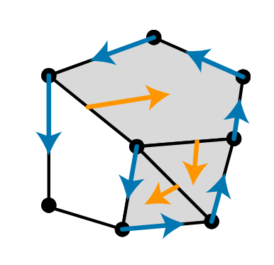
Definition. Let \(V\) be a discrete vector field. A \(V\)-path \(\Gamma\) from a cell \(\sigma_0\) to a cell \(\sigma_r\) is a sequence \((\sigma_0, \tau_0, \sigma_1, \dots, \tau_{r-1}, \sigma_r)\) of cells such that for every \(0\le i\le r-1:\)
$$
\sigma_i \text{ is a face of } \tau_i \text{ with } (\sigma_i, \tau_i \in V) \text{ and } \sigma_{i+1} \text{ is a face of } \tau_i \text{ with } (\sigma_{i+1}, \tau_i)\notin V.
$$\(\Gamma\) is closed if \(\sigma_0=\sigma_r\), and nontrivial if \(r>0\).
Definition. A discrete vector field V is a discrete gradient vector field if it contains no nontrivial closed V-paths.
Finally, with this in mind, we can define what properties should a Morse function satisfy on a given simplicial complex \(K\).
Definition. A function \(f: K\rightarrow \mathbb{R}\) on the cells of a complex K is a discrete Morse function if there is a gradient vector field \(V_f\) such that whenever \(\sigma\) is a face of \(\tau\) then
$$
(\sigma, \tau)\notin V_f \text{ implies } f(\sigma) < f(\tau) \text{ and } (\sigma, \tau)\in V_f \text{ implies } f(\sigma)\ge f(\tau).
$$\(V_f\) is called the gradient vector field of \(f\).
Definition. Let \(V\) be a discrete gradient vector field and consider
the relation \(\leftarrow_V\) defined on \(K\) such that whenever \(\sigma\) is a face of \(\tau\) then
$$
(\sigma, \tau)\notin V \text{ implies } \sigma\leftarrow_V \tau \text { and } (\sigma, \tau)\in V \text{ implies } \sigma\rightarrow_V \tau.
$$
Let \(\prec_V\) be the transitive closure of \(\leftarrow_V\) . Then \(\prec_V\) is called the partial order induced by V.
We are now ready to introduce one of the main theorems of discrete Morse Theory.
Theorem. Let \(V\) be a gradient vector field on \(K\) and let \(\prec\) be a linear extension of \(\prec_{V}\). If \(\rho\) and \(\psi\) are two simplices such that \(\rho \prec \psi\) and there is no critical cell \(\phi\) with respect to \(V\) such that \(\rho\prec\phi\preceq\psi\), then \(\kappa(\psi)\) collapses (homotopy equivalent) to \(\kappa(\rho)\).
Here, $$\kappa(\sigma) = closure(\cup_{\rho\in K; \rho\preceq\sigma}\rho)$$ an equivalent of sublevel set in the discrete setting.
This theorem says that given a gradient vector filed to a simplicial complex, and we consider how it is built over time by bringing each simplex in \(\prec\)’s order, then the topological changes happen only at the critical points determined by the gradient vector field. This strikingly is reminiscent of the case with the torus above.
This perspective is not only conceptually elegant but also computationally powerful: by identifying and retaining only the critical simplices, we can drastically reduce the size of our complex while preserving its topology. In fact, several groups of researchers have already utilized the discrete morse theory to simplify a function by removing topological noise.
Reference
- Bauer, U., Lange, C., & Wardetzky, M. (2012). Optimal topological simplification of discrete functions on surfaces. Discrete & computational geometry, 47(2), 347-377.
- Forman, R. (1998). Morse theory for cell complexes. Advances in mathematics, 134(1), 90-145.
- Scoville, N. A. (2019). Discrete Morse Theory. United States: American Mathematical Society.