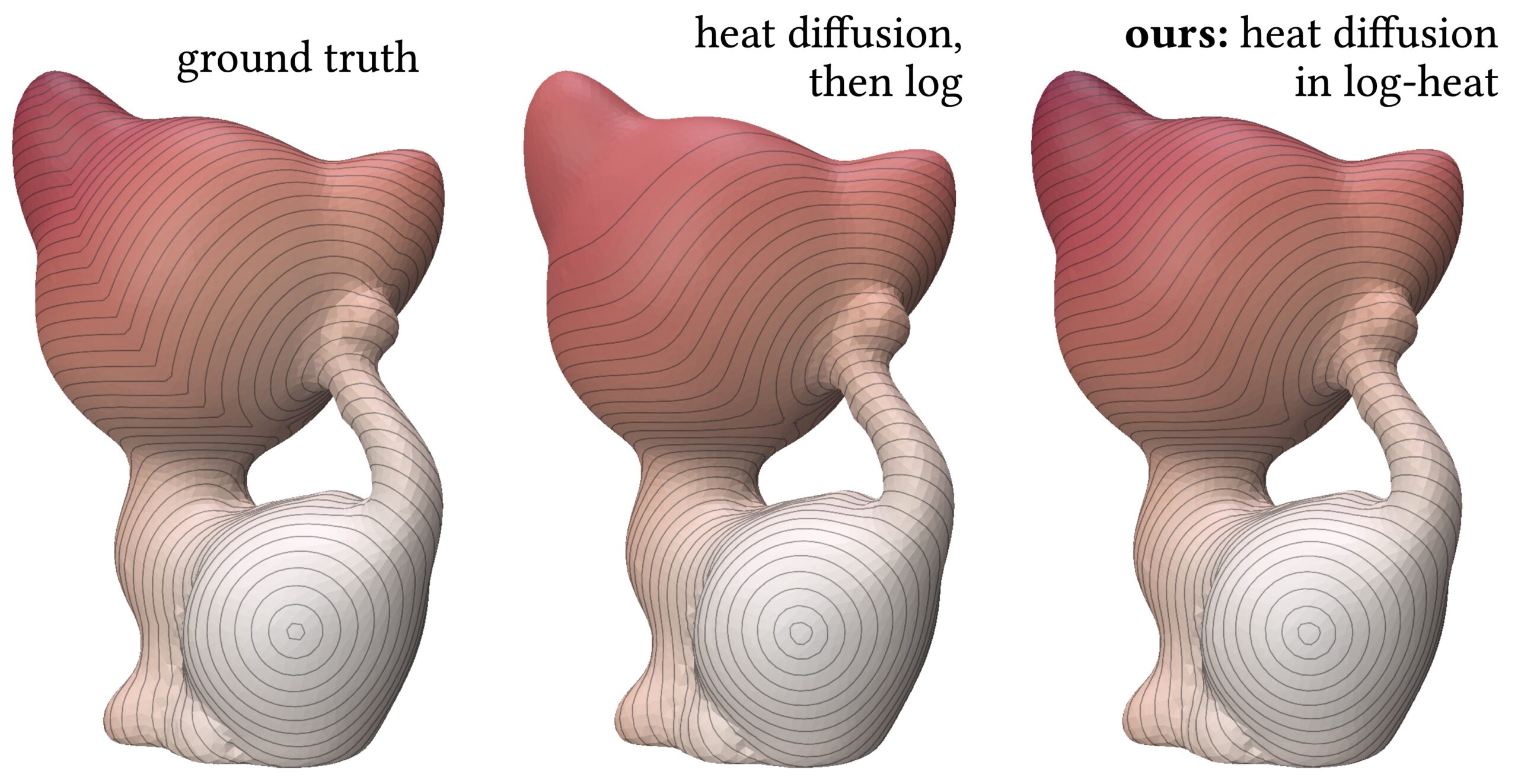
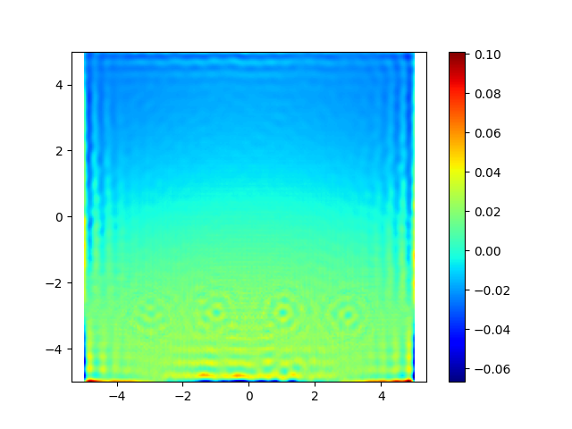
Figure 1: Comparison of distance estimation by heat methods. Standard diffuse-then-log (middle) suffers from numerical issues when the heat is small (large geodesic distances), leading to noisy and inaccurate isolines. Our proposed log-space diffusion (right) performs diffusion directly in the log-heat domain, producing smooth and accurate estimates, closely matching the ground-truth distances (left). It is worth noting that our solver outperforms others primarily for smaller time step values. This example was done at a time step of 0.01 with 50 time steps.
The heat equation is one of the canonical diffusion PDEs: it models how “heat” (or any diffusive quantity) spreads out over space as time progresses. Mathematically, let \(u(x,t) \in \mathbb{R}_{\geq 0}\) denote the temperature at spatial location \(x \in \mathbb{R}^{d}\) and time \(t \in \mathbb{R}\). The continuous heat equation is given by
\[\frac{\partial u}{\partial t} = \Delta u,\]
where \(\Delta u (x, t) = \sum_{i=1}^{d} \frac{\partial^2 u}{\partial x_i^2}\) is the Laplace operator representing how local temperature gradients drive heat from hotter to colder regions. On a surface mesh, the spatial domain is typically discretized so that the PDE reduces to a system of ODEs in time, which can be integrated using stable and efficient schemes such as backward Euler. Interestingly, in many applications—including geodesic distance computation 1 and optimal transport 2—it is often more useful to work with the logarithm of the heat rather than the heat itself. For example, Varadhan’s formula states that the geodesic distance \(\phi\) between two points \(x\) and \(x^*\) on a curved domain can be recovered from the short-time asymptotics of the heat kernel:
where \(k_{t,x^{*}}(x) = u(x,t)\) is the heat distribution at time \(t\) resulting from an initial Dirac delta at \(x^*\), i.e., \(u(x,0) = \delta(x-x^{*})\). In practice, this leads to a two-step workflow: (1) simulate the heat equation to obtain \(u_t\), and (2) take the logarithm to recover the desired quantity. However, this approach can be numerically unstable in regions where \(u\) is very small: tiny relative errors in \(u\) can be greatly magnified in the log domain. For example, an absolute error of \(10^{-11}\) in \(u\) becomes an error of roughly \(25.33\) in \(\log u\).
A natural idea is therefore to evolve the logarithm of the heat directly. Let \(u>0\) satisfy the heat equation and define \(w = \log u\). One can show that \(w\) obeys the nonlinear PDE 3
\[\frac{\partial w}{\partial t} = \Delta w + \|\nabla w\|_2^2.\]
This formulation has the appealing property that it avoids taking the logarithm after simulation, thereby reducing the amplification of small relative errors in \(u\) when \(u\) is tiny. However, the price of this reformulation is the additional nonlinear term \(\|\nabla w\|_2^2\), which complicates time integration as each step requires iterative optimization, and introduces a discrepancy with the discretized heat equation. In practice, evaluating \(\|\nabla w\|_2^2\) requires a discrete gradient operator, and the resulting ODE is generally not equivalent to the one obtained by first discretizing the heat equation for \(u\) (which involves only a discrete Laplacian) up to a log transform. This non-equivalence stems from (1) there is a new spatially discretized gradient operator, and (2) the fact that the logarithm is nonlinear and does not commute with discrete differential operators.
Motivated by this discrepancy, we take a different approach that preserves the exact relationship to the standard discretization. We first discretize the heat equation in space, yielding the familiar linear ODE system for \(u\). We then apply the transformation \(w = \log u\) to this discrete system, producing a new ODE for \(w\). Now, by construction, the new ODE is equivalent to the heat ODE up to a log transform of variable. This still allows us to integrate directly in log-space, which allows more accurate and stable computation. We show that this formulation offers improved numerical robustness in regions where \(u\) is very small, and demonstrate its effectiveness in applications such as geodesic distance computation.
Table 1: Side-by-side procedures for computing \(\log u\) in heat diffusion, note the highlighted steps are the same for standard heat diffusion and ours.
Standard (post-log)
Continuous log-PDE
Proposed discrete-log
1. Start with the heat PDE for \(u\).
1. Start with the log-heat PDE for \(w=\log u\).
1. Start with the heat PDE for \(u\).
2. Discretize in space \(\Rightarrow\) ODE for \(u\).
2. Discretize in space for \(\nabla\) and \(\Delta\) \(\Rightarrow\) ODE for \(w\).
2. Discretize in space \(\Rightarrow\) ODE for \(u\).
3. Time-integrate in \(u\)-space.
3. Time-integrate in \(w\)-space and output \(w\).
3. Apply change of variables \(w=\log u\) \(\Rightarrow\) ODE for \(w\).
4. Compute \(w=\log u\) as a post-process.
4. Time-integrate in \(w\)-space and output \(w\).
Background
We begin by reviewing how previous approaches are carried out, focusing on the original heat method 1 and the log-heat PDE studied in 3. In particular, we discuss two key stages of the discretization process: (1) spatial discretization, where continuous differential operators such as the Laplacian and gradient are replaced by their discrete counterparts, turning the PDE into an ODE; and (2) time discretization, where a numerical time integrator is applied to solve the resulting ODE. Along the way, we introduce notation that will be used throughout.
Heat Method
Spatial discretization. In the heat method 1, the heat equation is discretized on triangle mesh surfaces by representing the heat values at mesh vertices as a vector \(u \in \mathbb{R}^{|V|}\), where \(|V|\) is the number of vertices. A corresponding discrete Laplace operator is then required to evolve \(u\) in time. Many Laplacian discretizations are possible, each with its own trade-offs 4. The widely used cotangent Laplacian is written in matrix form as \(M^{-1}L\), where \(M, L \in \mathbb{R}^{|V| \times |V|}\). The matrix \(L\) is defined via
where \(i,j\) are vertex indices and \(\alpha_{ij}, \beta_{ij}\) are the two angles opposite the edge \((i,j)\) in the mesh. The mass matrix \(M = \mathrm{diag}(m_1, \dots, m_{|V|})\) is a lumped (diagonal) area matrix, with \(m_i\) denoting the area associated with vertex \(i\). Note that \(L\) has several useful properties: it is sparse, symmetric, and each row sums to zero. This spatial discretization converts the continuous PDE into an ODE for the vector-valued heat function \(u(t)\):
\[\frac{\mathrm{d}u}{\mathrm{d}t} = M^{-1}L\,u.\]
Time discretization and integration. The ODE is typically advanced in time using a fully implicit backward Euler scheme, which is unconditionally stable. For a time step \(\Delta t = t_{n+1} – t_n\), backward Euler yields:
\[(M – \Delta t\,L)\,u_{n+1} = M\,u_n,\]
where \(u_n\) is given and we solve for \(u_{n+1}\). Thus, each time stepping requires solving a sparse linear system with system matrix \(M – \Delta t\,L\). Since this matrix remains constant throughout the simulation, it can be factored once (e.g., by Cholesky decomposition) and reused at every iteration, greatly improving efficiency.
Log Heat PDE
Spatial discretization. In prior work 3 on the log-heat PDE, solving this requires discretizing not only the Laplacian term but also the additional nonlinear term \(\|\nabla w\|_2^{2}\). After spatial discretization, the squared gradient norm of a vertex-based vector \(w \in \mathbb{R}^{|V|}\) is computed as
where \(G_{k} \in \mathbb{R}^{|F| \times |V|}\) is the discrete gradient operator on mesh faces for the \(k\)-th coordinate direction, and \(W \in \mathbb{R}^{|V| \times |F|}\) is an averaging operator that maps face values to vertex values. With this discretization, the ODE for \(w(t) \in \mathbb{R}^{|V|}\) becomes
Time discretization and integration. If we apply fully implicit Euler, we would find \(w^{n+1}\) by solving a nonlinear equation. To avoid this large nonlinear solve, prior work 3 splits the problem into two substeps:
a linear diffusion part: \(\frac{\mathrm{d}w}{\mathrm{d}t} = M^{-1}L\,w\), which is stiff but easy to solve implicitly,
a nonlinear part: the full equation, which is nonlinear but convex.
This separation lets each component be treated with the method best suited for it: a direct linear solve for the diffusion, and a convex optimization problem for the nonlinear term. Using Strang-Marchuk splitting:
Full-step nonlinear term: Solve a convex optimization problem to find \(w^{(2)}\)
Half-step diffusion: \((M – \frac{\Delta t}{2} L)\,w^{(3)} = Mw^{(2)}\), and set \(w^{n+1} = w^{(3)}\)
A New ODE in Log-Domain
Let us revisit the spatially discretized heat (or diffusion) equation. For each vertex \(i \in \{1, \dots |V|\}\) on a mesh, its evolution is described by
where \(u\) represents our heat, and \(L\) is the discrete Laplacian operator. A key insight is that the Laplacian term can be rewritten as a sum of local differences between a point and its neighbors:
\[(Lu)_i = \sum_{j \sim i}L_{ij} (u_j – u_i).\]
This shows that the change in \(u_i\) depends on how different it is from its neighbors, weighted by the Laplacian matrix entries. Now, before doing time discretization, we use a change of variable \(w \Leftarrow\log u\), accordingly, \(u = \mathrm{e}^{w}\), to obtain the ODE
In vectorized notation, we construct a matrix \(\tilde{L} \Leftarrow L – \mathrm{diag}(L_{11}, \dots, L_{|V| \,|V|})\), which zeros out the diagonals of \(L\). Then the log heat \(w(t) \in \mathbb{R}^{|V|}\) follows the ODE
This ODE is equivalent to the standard heat ODE up to a log transform of the integrated results, but crucially it avoids the amplification of small relative errors in \(u\) when \(u\) is tiny by integrating directly in log-space.
Numerical Solvers for Our New ODE
Forward (Explicit Euler)
The most straightforward approach uses explicit Euler to update the solution at each time step. The update rule is
It can be shown that minimizing the objective function
\[f(w) = \sum_{i}M_iw_i\]
with the inequality constraint defined above yields the exact solution to the original equation. We have written a complete proof for this finding here. We implement this constrained optimization problem using the Clarabel solver 6 in CVXPY 7, a Python library for convex optimization problems.
Experiments
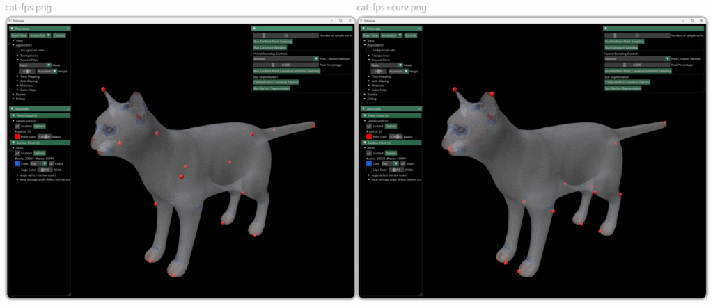
As mentioned earlier, the log heat equation is widely used to efficiently approximate geodesic distances. To evaluate our method, we selected a point on each mesh as a heat source and computed approximate geodesic distances from that point using the log-heat solution with Varadhan’s formula. For comparison, all solvers were applied within the same log-heat framework described in Equation 2 and tested on meshes of varying complexity. As ground truth, we used libigl’s 5 implementation of exact discrete geodesic distances. All experiments used 10 diffusion time-steps equally spaced between \(t = 0\) and \(t = 10^{-2}\). The results are shown in Table 2.
Table 2: Correlation analysis results.
Mesh
# of verts
Method
Pearson \(r\) ↑
RMSE ↓
MAE ↓
Lilium
3389
HeatBackward
0.992
0.267
0.207
LogHeatBackward
0.653
0.510
0.385
NewLogHeatBackward (ours)
0.997
0.070
0.063
Cat
9447
HeatBackward
0.991
0.063
0.043
LogHeatBackward
0.513
0.531
0.474
NewLogHeatBackward (ours)
0.998
0.150
0.140
Spot
11533
HeatBackward
0.992
0.318
0.248
LogHeatBackward
0.382
0.982
0.853
NewLogHeatBackward (ours)
0.994
0.121
0.115
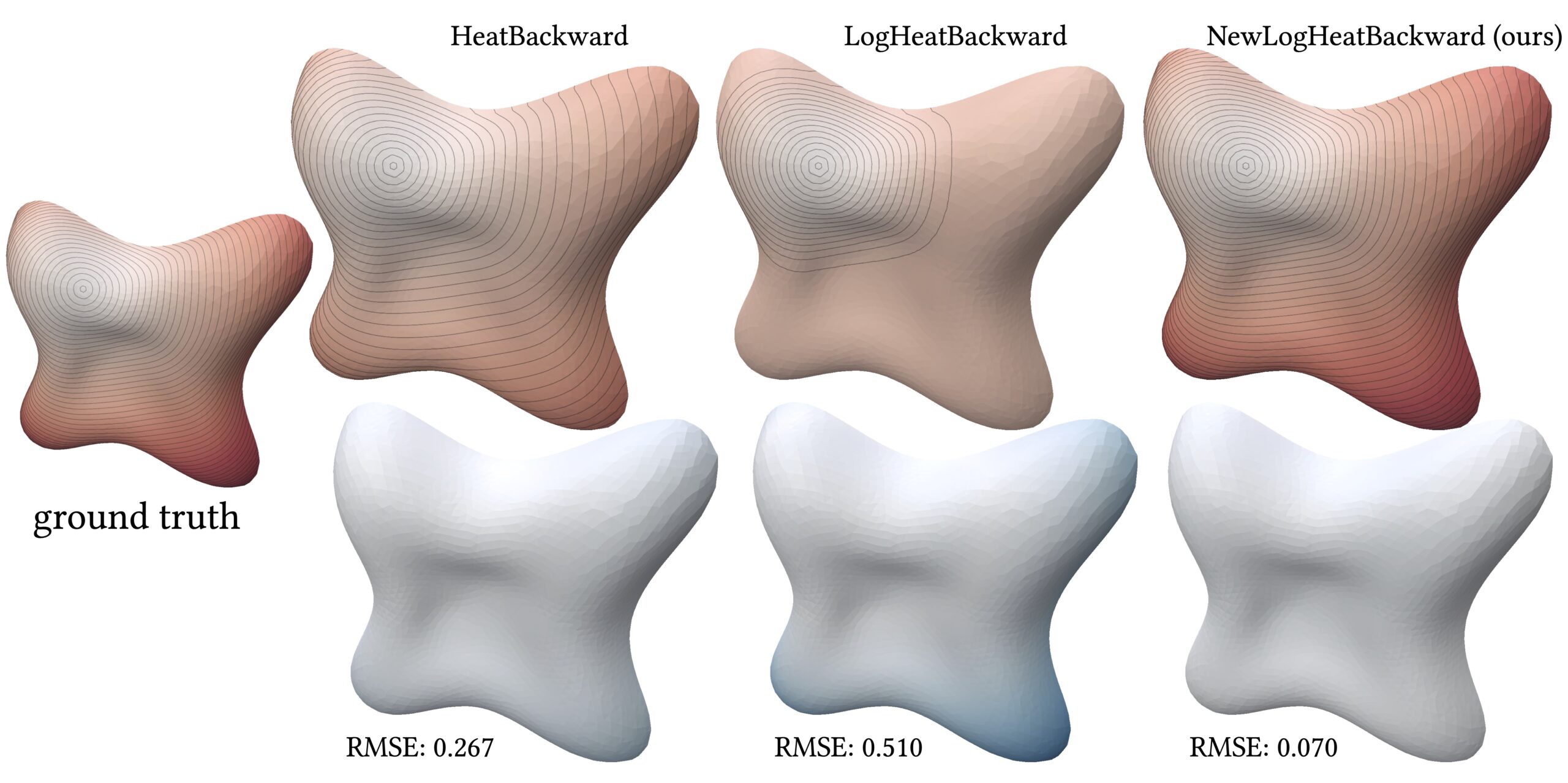
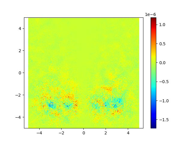
Figure 2: Comparison of geodesic distance computation on the Lilium mesh (top) and the corresponding error relative to the ground-truth distances (bottom).
Our method, NewLogHeatBackward, consistently outperforms HeatBackward and LogHeatBackward on all tested meshes, showing the highest correlation with the ground truth while maintaining low RMSE and MAE. This demonstrates that it provides more accurate and reliable approximations of geodesic distances across meshes of different sizes and complexities. While performance can still vary depending on the mesh, NewLogHeatBackward performs especially well on well-behaved meshes, as shown in Figure 2. Figure 3 further illustrates its accuracy by comparing the exact geodesic distances with those computed by each solver. Although the method may slightly overshoot in some cases, it consistently produces results closest to the true geodesic distances.
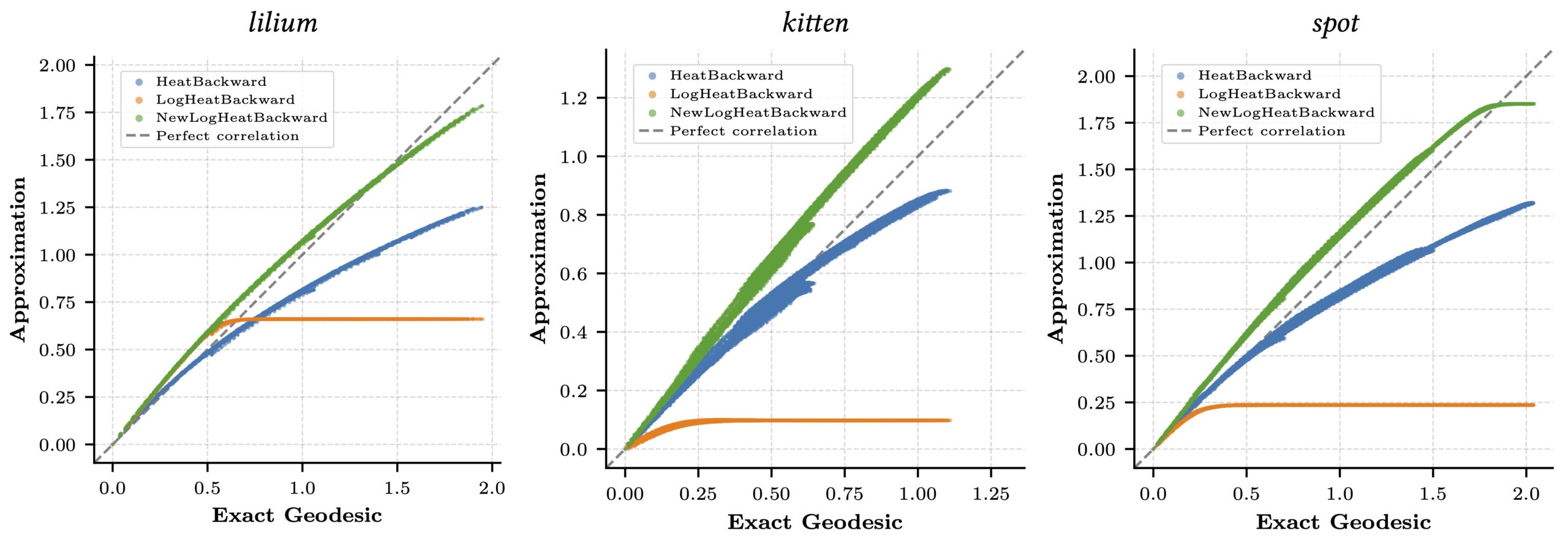
Figure 3: Correlation plot for log heat methods against an exact geodesic computation.
In Figure 1, the flat region for the NewLogHeatBackward Solver probably indicates regions of numerical overflow/underflow, since the log of tiny heat values is going to be incredibly negative. Through our experimentation we observed that the solver for this our formulated PDE outperforms others mostly in cases where the diffusion time-step is extremely small.
References
[1] Keenan Crane, Clarisse Weischedel, and Max Wardetzky. “The Heat Method for Distance Computation.” Communications of the ACM, vol. 60, no. 11, October 2017, pp. 90–99.
[2] Justin Solomon, Fernando de Goes, Gabriel Peyré, Marco Cuturi, Adrian Butscher, Andy Nguyen, Tao Du, and Leonidas Guibas. “Convolutional Wasserstein Distances: Efficient Optimal Transportation on Geometric Domains.” ACM Transactions on Graphics, vol. 34, no. 4, August 2015.
[3] Leticia Mattos Da Silva, Oded Stein, and Justin Solomon. “A Framework for Solving Parabolic Partial Differential Equations on Discrete Domains.” ACM Transactions on Graphics, vol. 43, no. 5, October 2024.
[4] Max Wardetzky, Saurabh Mathur, Felix Kälberer, and Eitan Grinspun. “Discrete Laplace Operators: No Free Lunch.” In Proceedings of the Fifth Eurographics Symposium on Geometry Processing, pages 33–37, Barcelona, Spain, 2007.
[5] Alec Jacobson et al. “libigl: A Simple C++ Geometry Processing Library.” Available at https://github.com/libigl/libigl, 2025.
[6] Paul J. Goulart and Yuwen Chen. “Clarabel: An Interior-Point Solver for Conic Programs with Quadratic Objectives.” arXiv preprint arXiv:2405.12762, 2024.
[7] Steven Diamond and Stephen Boyd. “CVXPY: A Python-Embedded Modeling Language for Convex Optimization.” Journal of Machine Learning Research, vol. 17, no. 83, pages 1–5, 2016.
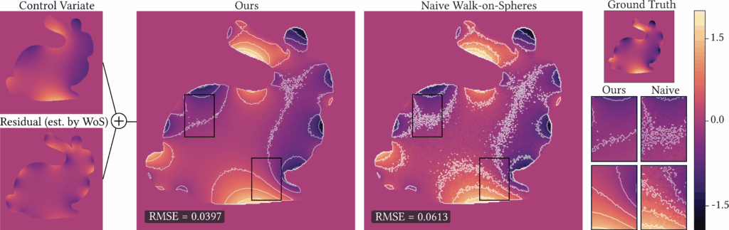
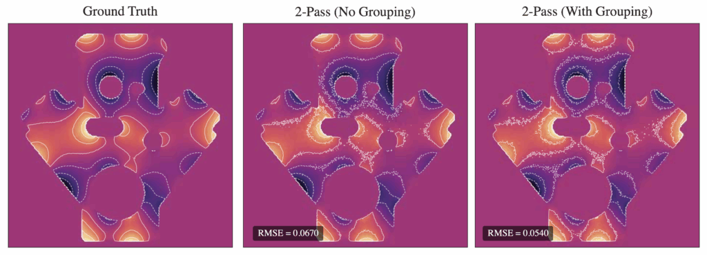
Figure 1. Our method reduces the variance of the Walk-on-Spheres algorithm with minimal computational overhead. We compute a harmonic control variate, apply Walk-on-Spheres to the residual, and sum the results to obtain the final solution. With 256 walks, our approach (left) achieves a substantial reduction in RMSE compared to the standard method (right).
1 Introduction
A classic problem in computer graphics is the interpolation of boundary values into a region’s interior. More formally, given a domain \( \Omega \) and values prescribed on its boundary \( \partial \Omega \), we seek a smooth function \( u: \mathbb{R}^n \to \mathbb{R} \) that satisfies the boundary value problem
$$\begin{align} \Delta u(x) = 0 \text{ in } \Omega, \ \quad u(x) = g(x) \text{ on } \partial \Omega, \end{align}$$
where \(g(x)\) is a given boundary function. This is the well-known Laplace’s equation with Dirichlet boundary conditions. A standard approach for solving such PDEs is the finite element method (FEM), which discretizes the domain into a mesh and computes a weak solution. However, the accuracy of FEM depends critically on the quality of the mesh and how well it approximates the domain geometry. In contrast, Monte Carlo methods offer an appealing alternative — particularly the walk on spheres (WoS) algorithm [Muller, 1956], which avoids meshing altogether. WoS exploits the Mean Value Property of harmonic functions (i.e., functions satisfying \( \Delta u = 0) \), which states:
for any ball \( B(x, r) \subseteq \Omega \). This property implies that \( u(x) \) can be estimated by recursively sampling points on the boundary of spheres centered at \( x \), continuing until a point lands on \( \partial \Omega \), where the value is known from \( g(x) \). Compared to FEM, WoS scales much better with geometric complexity and does not require certain properties of the mesh like watertightness, free of self-intersections, manifoldness, etc. While WoS does not generalize to all classes of PDEs, it offers many advantages even beyond geometric robustness (See Sawhney and Crane 2020, Section 1).
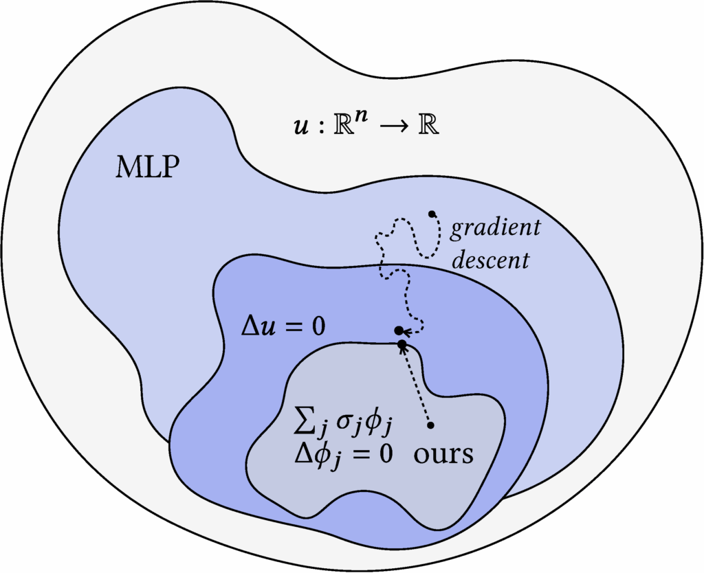
While WoS is an unbiased estimator and is largely agnostic to geometric quality, it can suffer from high variance, often requiring many samples to converge and thus incurring high computational cost. A common way to reduce variance is to use a control variate, and prior work has explored applying them to WoS. The main challenge in using control variates is finding a suitable reference function (one with a known integral) that also closely matches the target function. One research direction to address this challenge is neural control variates—constructing the control variate function using neural networks (See Li et al. 2024, who applied this approach to WoS). While their method leverages a clever technique known as automatic integration [Li et al. 2024] to perform closed-form integration, it still suffers from substantial overhead during both training and inference due to the use of MLPs. In contrast, we propose harmonic control variates, where harmonicity is built into the control variate representation by design, enabling closed-form integration directly as a function evaluation. Moreover, our representation is fitted using a simple least squares procedure, which is significantly more efficient than training a neural network via gradient descent. It also allows for much faster evaluation at inference time.
Specifically, our approach consists of two main steps. (1) We construct a harmonic representation as a weighted sum of harmonic kernels (e.g., Green’s functions), and fit the weights/coefficients using a sparse set of points in the domain along with their WoS-based estimates. This fitting reduces to solving a linear system of the form \( \Phi \sigma = u \) for the weight vector \( \sigma \). The resulting function is harmonic by construction, and although it provides a useful denoised estimate, it remains biased with respect to the true solution \( u(x) \) almost everywhere in the domain. (2) To correct for this bias, we use the harmonic representation as a control variate, thus termed harmonic control variate. Because the representation is harmonic, its mean over any sphere can be computed in closed form via simple function evaluation. We then define a residual Laplace problem, where the boundary condition is the difference between the true boundary data and our representation. Solving this residual problem with WoS and adding the result back to the harmonic representation yields an unbiased estimator for \( u(x) \). This control variate estimator reduces variance whenever the representation closely approximates \( u(x) \) on the boundary.
Our harmonic control variate achieves significant variance reduction compared to naive WoS across a range of geometries, yielding an average 40% reduction in RMSE compared to the naive baseline at 128 walks. In addition to its effectiveness, our method is simple to implement: the entire pipeline can be reproduced in Python with minimal code, leveraging just a few function calls to the underlying integrated C++ library Zombie [Sawhney and Miller 2023]. To illustrate its flexibility, we also extend our approach to settings with Neumann boundary conditions and with an alternative Monte Carlo scheme Walk on Stars [Sawhney, Miller, et al. 2023]. We believe that this classically inspired yet practical control variate representation (a sum of harmonic kernels) offers useful insights for the broader computational science and graphics communities.
Figure 2. Finding a suitable control variate function, ours vs. MLP
2 Background
2.1 Walk on Spheres
The Walk on Spheres (WoS) algorithm [Muller 1956] can be motivated in two complementary ways. One is via Kakutani’s principle, which states that the solution value \( u(x) \) of a harmonic function at any point \( x \in \Omega \) is equal to the expected boundary value \( u(x) = \mathbb{E}[g(y)] \), where \( y \in \partial \Omega \) is the first boundary point reached by a Brownian motion starting at \( x \). We focus on a second, more constructive motivation coming from the mean value property of harmonic functions (see eq. (*)). This property immediately suggests a single-sample Monte Carlo estimator:
where \( \mathscr{U}(\partial B(x,r)) \) denotes the uniform distribution on the sphere of radius \( r \) centered at \( x \). Specifically, the mean value property suggests that this estimator is unbiased:
where \( p(y) = 1/|\partial B(x,r)| \) denotes the uniform probability density on \( \partial B(x, r) \).
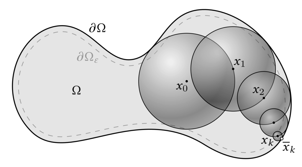
However, the difficulty is that \( u(y) \) is unknown unless \( y \) lies on the boundary \( \partial \Omega \). To address this, the mean value property is applied recursively: each sampled point becomes the new center for the next sphere, and the process continues until the boundary is reached. Since naïve recursion would never terminate, the algorithm introduces a tolerance \( \epsilon \). Specifically, once a point \( x_k \) lies within distance \( \epsilon \) of the boundary, we project it to the nearest boundary point \( \bar{x}_k \in \partial \Omega \) and evaluate the boundary condition \( g(\bar{x}_k) \). This serves as the base case of the recursion.
Formally, letting \( \Omega_\epsilon \) denote the \( \epsilon\)-shell adjacent to the boundary (illustrated in Figure 3), the recursive rule is
with the next sample \( x_{k+1} \sim \mathscr{U}(\partial B(x_k, r_k)) \), where \( r_k \) is the largest radius such that the ball remains fully contained in \( \Omega \). As the recursion telescopes, the final estimator is simply
where each \( \bar{x}_{n_i}^{(i)} \in \partial \Omega \) is the endpoint of the \( i \)-th walk, reached on its \( n_i \)-th step. This estimator remains unbiased as \( \epsilon \to 0 \), but its efficiency is governed by the variance of the boundary condition \( g(x) \). In fact, the variance of the estimator is directly proportional to that of \( g(x) \):
Intuitively, if \( g(x) \) varies significantly across the boundary region where walks terminate, the estimates \( \langle u(x_0) \rangle \) will fluctuate sharply between different exit points, leading to a noisy approximation of the solution. Conversely, if \( g(x) \) is nearly constant around the relevant boundary region, most walks yield similar values, and the estimator stabilizes. This observation is central to our two-pass variance-reduction strategy (see Section 3.2).
2.2 Control Variates
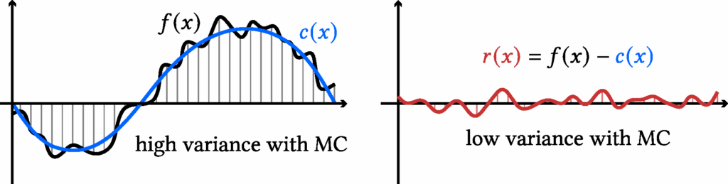
To build intuition, let us first consider the simple task of integrating a scalar function in one dimension. Suppose we want to estimate
$$\begin{align} F = \int_{a}^{b} f(x)\, \mathrm{d}x, \end{align}$$
using Monte Carlo (MC) sampling. A naive single-sample Monte Carlo estimator is
$$\begin{align} \langle F \rangle = |b-a|\, f(x), \quad x \sim \mathscr{U}[a,b]. \end{align}$$
The idea of a control variate is to introduce a function (c(x)) that (i) closely approximates (f(x)) and (ii) has a known closed-form integral, denoted (C). We can rewrite the target integral as
This yields a single sample Monte-Carlo estimator with control variate:
$$\begin{align} \langle F \rangle^{(\text{cv})} = |b-a| \big(f(x) – c(x)\big) + C, \quad x \sim \mathscr{U}[a,b]. \end{align}$$
It is clear that it remains unbiased. Moreover, it achieves lower variance whenever the residual \( r(x) := f(x) – c(x) \) is less variable than the original function \( f(x) \):
$$\begin{align} \mathrm{Var} [\langle F \rangle^{(\text{cv})} ] < \mathrm{Var}[\langle F \rangle] \quad \iff \quad \mathrm{Var}[f(x) – c(x)] < \mathrm{Var}[f(x)]. \end{align}$$
Figure 4. An illustration of control variate reducing Monte Carlo estimation variance in 1D.
Control Variates for Walk-on-Spheres. Motivated by this principle, prior work [Li et al. 2024] incorporated control variates directly into the mean value formulation of WoS. At each step of the walk, they replace the boundary condition with a residual correction, and by eq. (*),
where \( C(x) = \frac{1}{\lvert \partial B(x,r)\rvert}\int_{\partial B(x,r)} c(y)\,\mathrm{d}y \) and \( c : \mathbb{R}^d \to \mathbb{R} \) is the control variate. This introduces the challenge of designing a control variate \(c\) that is both expressive and admits a tractable integral \(C(x)\). Li et al. [2024] addressed this by parameterizing \( c \) with a neural network and using automatic integration to evaluate \(C(x)\). However, this approach requires costly neural network evaluations at every step of the walk and additional training via gradient descent. In contrast, we take the insight that if \( c \) is also harmonic, then \( C(x) = c(x) \) by eq. (*). Our method only evaluates the control variate twice per walk and fits it directly via least squares, making it significantly more efficient while still achieving variance reduction.
3 Method
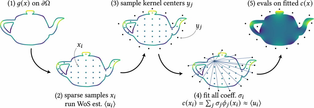
Our method introduces a harmonic representation that serves as a control variate for variance reduction. We first describe the formulation of this harmonic representation and how it can be efficiently solved in Section 3.1. Next, we explain how this representation functions as a control variate to reduce variance in Monte Carlo estimation in Section 3.2. Finally, we present implementation details in Section 3.3. An overview of our method is illustrated in Figure 5.
3.1 Mixture of Harmonic Kernels Representation
We propose a simple, kernel-based representation for approximating a target harmonic function \( u(x) \), subject to Dirichlet boundary conditions \( u(x) = g(x) \) on \( \partial \Omega \). Specifically, we approximate \( u(x) \) using a mixture of harmonic kernels \( \phi_j(\,\cdot\,) \):
where each \( \phi_j(x) \) is itself harmonic. By linearity, the mixture \( c(x) \) is also harmonic. To ensure that \( c(x) \) remains free of singularities inside the domain \( \Omega \), the kernels are chosen carefully. The coefficients \( \{\sigma_j\}_{j=1}^M \) are free parameters that must be fitted to approximate \( u(x) \).
There are many possible choices of harmonic kernels. A canonical example in two dimensions is the Green’s function,
where the centers \( \{y_j\} \) are placed outside of \( \Omega \) to avoid singularities within the domain. We will introduce another kernel choice in Section 4.
Fitting the coefficients: To determine the coefficients \( \sigma_j \), we first sample a sparse set of interior points \( \{x_i\}_{i=1}^N \subset \Omega \). At each point, we estimate \( \langle u(x_i) \rangle \) using Walk-on-Spheres (WoS), which leverages the known boundary condition. This produces training tuples \( \{(x_i, \langle u(x_i) \rangle) \}_{i=1}^N \), where \( c(x_i) \) should approximate \( \langle u(x_i) \rangle \). Each tuple gives a linear constraint on \( \sigma_j \), leading to the linear system:
such that we can introduce some regularization terms (see Section 3.3). An example of this fitting procedure using the Green’s kernel is illustrated in Figure 6.
Figure 5. An overview of our method.
Figure 6. The fitting process of our mixture of kernels representation 𝑐 (𝑥).
Intuitively, this representation projects the set of sparse and noisy estimates of \( u(x_i) \), i.e., the vector \( \langle u \rangle \), onto the subspace spanned by the harmonic kernels \( \{\phi_j(x)\} \). Since this fit is based only on a limited set of points and kernels and does not enforce correctness elsewhere, this representation is a biased estimator. Therefore, while this representation \( c(x) \) serves as a useful denoiser due to the smoothness of the kernels, it is not a sufficiently accurate approximation of the true solution \( u(x) \), see Figure 5. In the next section, we show how it can be leveraged as a control variate to reduce variance and obtain an unbiased estimate of \( u(x) \) throughout \( \Omega \).
3.2 Two-Pass with Control Variates
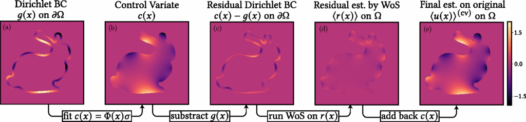
The main advantage of our representation \( c(x) \) being harmonic is that it satisfies \( \Delta c(x) = 0 \) in \( \Omega \). This allows us to define a residual PDE:
which corresponds to solving for the harmonic residual function \( r(x) := u(x) – c(x)\). Since the Dirichlet boundary condition for \( r(x) \) is known, namely \( r(x) = g(x) – c(x) \) on \( \partial \Omega \), we can apply the Walk-on-Spheres (WoS) algorithm to estimate \( \langle r(x) \rangle \). Our control variate estimator for \( u(x) \) is then given by
The argument for why this estimator is still unbiased and has smaller variance is similar to the 1D case outlined in Section 2.2. This estimator is unbiased since
where we used the fact that \( \mathbb{E}[\langle r(x) \rangle] = r(x) \) due to the unbiasedness of WoS. Therefore, as the number of random walks increases, the control variate estimator \( \langle u(x) \rangle^{(\text{cv})} \) converges to the true solution \( u(x) \). For variance reduction, observe that
As discussed earlier in the end of Section 2.1, variance is reduced when \( c(x) \) provides a good approximation to \( u(x) \) on the boundary. In this case, the residual boundary condition \( g(x) – c(x) \) has a smaller range, resulting in reduced variance in the WoS estimates for \( r(x) \) and, by extension, for \( u(x) \).
3.3 Implementation Details
We next describe several implementation choices in setting up and solving the linear system, as well as in implementing control variates.
Linear System Setup. Our formulation yields an \( N \times M \) linear system, where \( N \) is the number of constraints (sampled interior points) and \( M \) is the number of kernels. We deliberately set \( N > M \), making the system over-constrained. This avoids ill-posedness and eliminates the possibility of infinitely many solutions. To further enhance stability, we adopt Kd-tree based adaptive sampling, which distributes interior points evenly across the domain rather than allowing clusters in small regions. This reduces the risk of nearly colinear rows in the system matrix, which would otherwise harm numerical conditioning. Finally, we add regularization to eq. (***) to improve robustness near the boundary. Without it, the fitted representation tends to produce large coefficient magnitudes, leading to spikes and non-smooth artifacts. We experimented with both \( \ell_2 \) (ridge) regularization, which discourages large weights, and \( \ell_1 \) (lasso) regularization, which can additionally drive coefficients to zero. Both were effective, but we ultimately used \( \ell_2 \) in our experiments.
Control Variates with Zombie [Sawhney and Miller 2023].We build on the Zombie library, which provides efficient C++ implementations of Monte Carlo geometry processing methods along with Python bindings. In the baseline setting, Zombie takes as input the geometry together with boundary conditions sampled on a grid. During Walk-on-Spheres (WoS), Zombie interpolates these grid values whenever a trajectory hits the boundary, and then outputs estimated interior values on a user-specified grid resolution. Our variance reduction technique using control variates requires only a minimal change to this setup. Instead of supplying the original boundary condition, we provide the boundary condition of the residual function. Zombie then performs WoS to estimate the residual inside the domain. The final solution is obtained by simply adding back the evaluation of \( c(x) \) on the grid to these residual estimates. This simple modification makes the method straightforward to implement while still delivering effective variance reduction.
4 Experiments
We explore two types of harmonic kernels for our harmonic representation. The first is the 2D fundamental solution (Green’s function): for \( x,y\in\mathbb{R}^2 \),
which satisfies \( \Delta_x G^{\mathbb{R}^2}(x,y)=\delta(x-y)\) and thus harmonic in \(x\) away from the singularity at \(y\); it underlies methods such as the Mixture of Fundamental Solutions and boundary-element approaches.
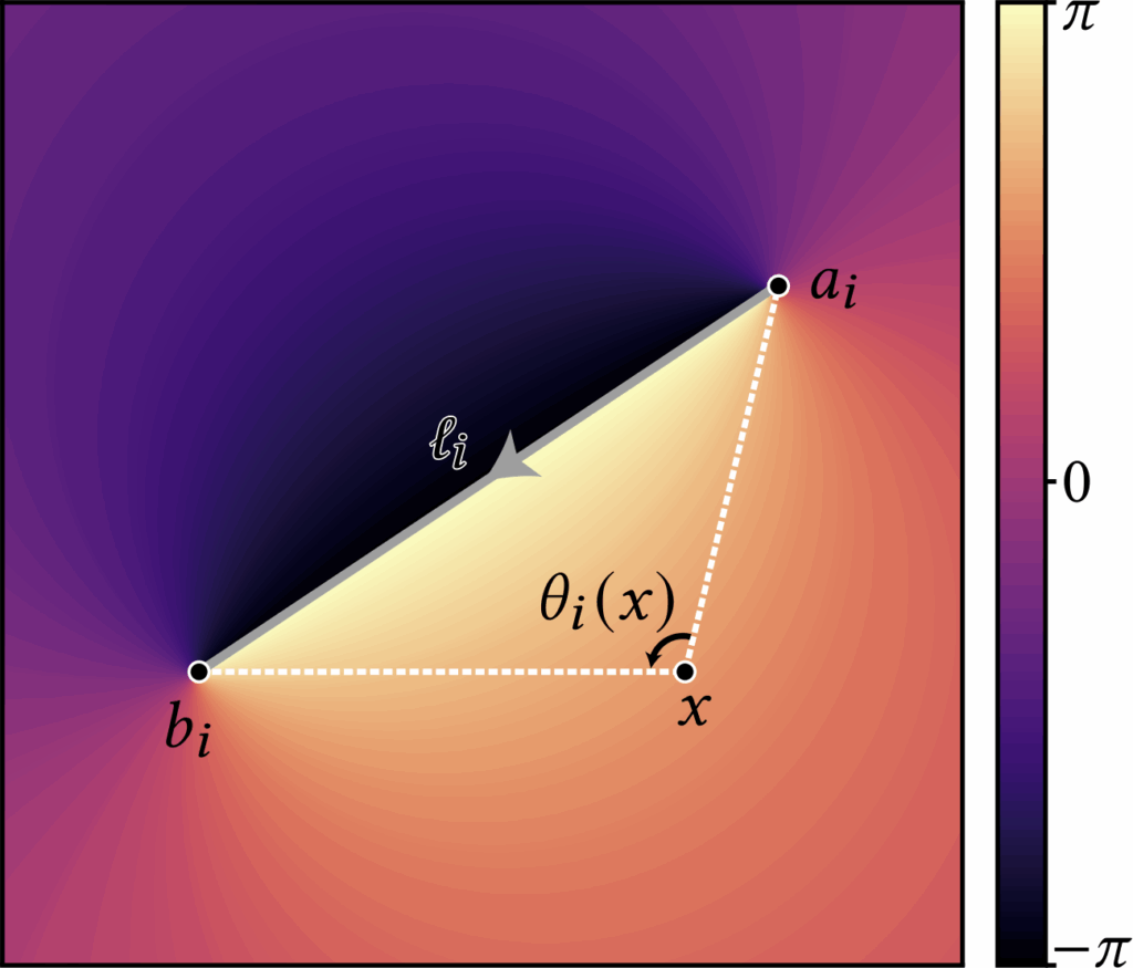
The second is the angle kernel obtained by integrating an angular density along a directed curve. For 2D polylines, the kernel admits a closed form: writing the (i)-th directed segment as \( \ell_i=[a_i,b_i] \), the associated angle kernel is defined as
with \( \det(u,v)=u_1v_2-u_2v_1 \). The \( \operatorname{atan2} \) formulation is numerically robust and returns the signed angle in \((-\pi,\pi]\). One can verify that the kernel is harmonic for \(x\notin\ell_i\); across the segment the angle exhibits \(\pm 1\) jump discontinuities. This angle representation is inspired by generalized winding-number and boundary-integral formulations (see Jacobson, Kavan, and Sorkine [2013])
Figure 7. The angle kernel associated with a line segment
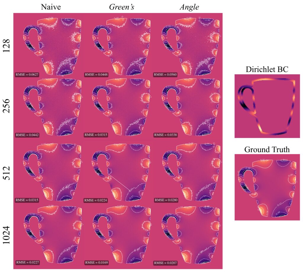
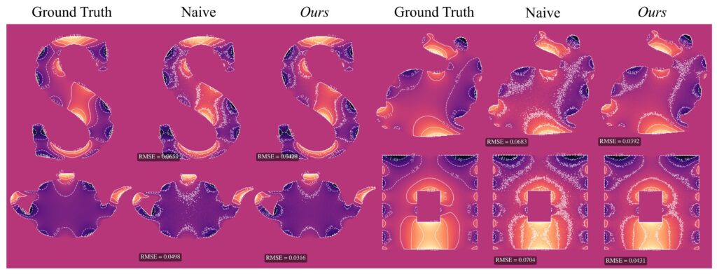
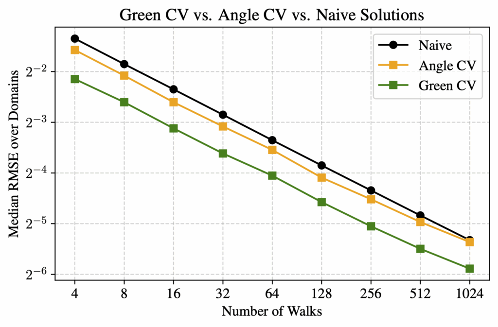
To verify our 2-pass method, we compared it against a reference solution obtained by running WoS with 32,768 walks, which we take as ground truth since this number is sufficient for convergence. For evaluation, we tested using between 4 and 1024 walks, and compared three methods—naive WoS, control variates with the Green’s function, and control variates with the angle kernel. We measured the median RMSE across 20 unique domains relative to the reference solution.
For all experiments, we used the following settings. The grid resolution was \( 256 \times 256 \) and the epsilon shell for WoS was \( 0.001 \). The number of basis functions for the denoiser was \( 80 \) and the number of walks for the samples for the denoisers was \( 128 \). We used \( \ell_2 \) regularization with \( \alpha = 0.1 \). The Dirichlet boundary condition we used is given by:
Figure 8a. Comparing Green’s kernel vs. Angle kernel against naive WoS, on a single domain with varying number of walks.
Figure 8b. Comparing our method vs. naive WoS for a variety of domains. We used Green’s kernel and 256 walks.
Based on RMSE, we observed that our control variate method for both kernels outperformed the naive WoS on average. The control variate with Green’s theorem showed significant linear improvement as the number of walks increased. The angle kernel did not yield as good results as Green’s; however, in the vast majority of experiments, the angle kernel control variate still achieved better RMSE than naive WoS. The only exception we observed was on more complex domains with a high number of walks. In contrast, for the Green’s kernel, we did not encounter any domain or walk count in which naive WoS outperformed the control variate method.
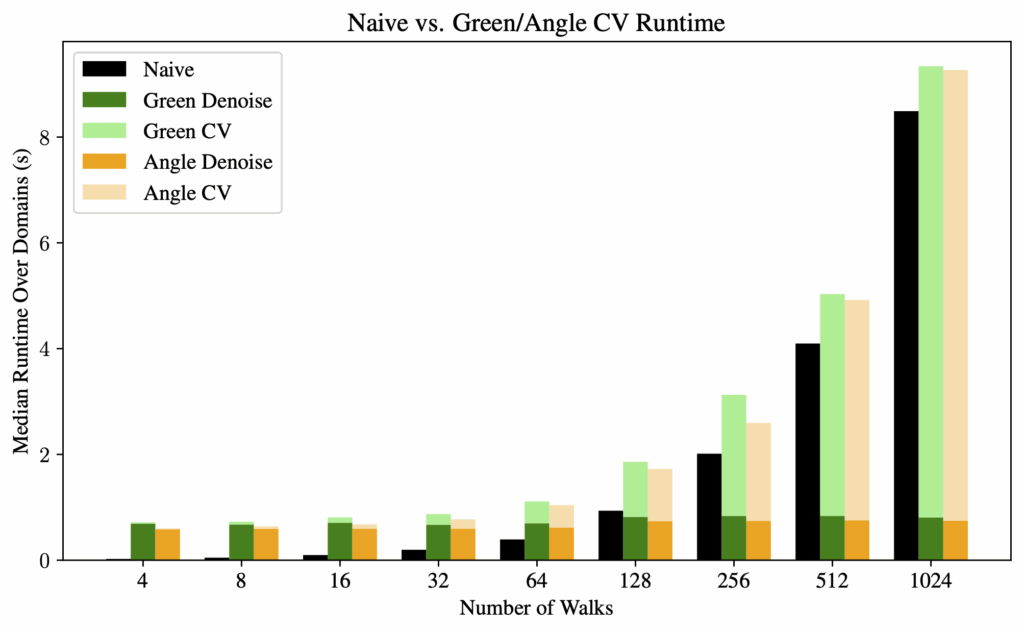
For computation time, we observed that the denoising process has a fixed amount of overhead. Therefore, as the number of walks increases, the denoising time becomes a negligible factor in the overall computation time. The bottleneck is then essentially the same as the naive method: the random walks.
Figure 9. RMSE comparing different kernels, varying the number of walks
Figure 10. Runtime comparison between naive WoS and our harmonic control variate method
5 Extensions
5. 1 N-Pass Gradient Descent Approach
Building upon the 2-pass harmonic control variate method, we experimented with an n-pass gradient descent approach to iteratively refine the control variate using Monte Carlo estimates as supervision. This method was motivated by the Neural Walk-on-Spheres framework [Nam, Berner, and Anandkumar 2024], which uses a general-purpose neural network \( u_\theta(x) \) as the learned control variate. Our method instead optimizes the coefficient weights \( \sigma ∈ ℝ^{M} \) of a harmonic control variate \( c(x) \), adhering to the structure of the underlying PDE.
The weights \( \sigma \) are initialized from a small set of sample points via the linear system (**), and stochastic gradient descent aims to then minimize the discrepancy between the control variate \( c(x) \) and Monte Carlo estimates \( \langle u(x) \rangle \).
Our optimization loop is implemented as follows:
Sample a batch of interior points \( x_i \) and compute Monte Carlo estimates \( \langle u(x_i) \rangle \) for each batch point using WoS
Evaluate the current control variate at each \( x_i \), and compute the mean square error (MSE) loss $$\mathscr{L} = \frac{1}{B} \sum_{i=1}^{B} \left( c(x_i) – \langle u(x_i) \rangle \right)^2$$
Perform a gradient step on \( \mathscr{L} \) with respect to \( \sigma \) via Adam optimizer
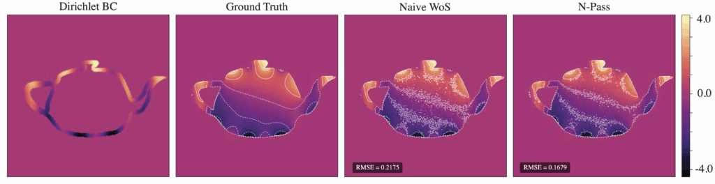
Figure 11. Naive WoS with 64 walks, 65536 points vs. n-pass with 32 pts/batch, 512 learning steps, 128 walks per sample pt., 32 walks in residual, Green’s function, learning-rate=0.01
For the same total number of walks, Figure 11 illustrates a significant improvement in RMSE compared to naive WoS, with the contours indicating a much less noisy interpolation of the boundary for our n-pass solution.
Further improvements include accelerating the repeated computation of \( c(x) \), adaptively adjusting the learning rate, and experimenting with different weight initializations. For example, when artifacts appeared in the denoiser due to a large number of monopoles, these artifacts remained present even after the optimization, since weights were initialized based on the denoiser.
5.2 Neumann Boundary Conditions
Many real-world PDE problems involve boundary behavior that is best described by flux, rather than a set of fixed values. Neumann conditions prescribe the normal derivative of the solution along the boundary. In the case of mixed boundary conditions, we seek a function \( u \) satisfying:
$$ \Delta u = 0 \text{ in } \Omega, \quad u = g \text{ on } \partial\Omega_D, \quad \frac{\partial u}{\partial n} = h \text{ on } \partial\Omega_N $$
where the boundary \( \partial \Omega = \partial \Omega_D \cup \partial\Omega_N \) is partitioned into Dirichlet and Neumann components. A 2-pass approach in this setting would first construct a control variate \( c(x) \approx u(x) \), and estimate the residual \( u(x) – c(x) \) which satisfies:
$$\Delta(u – c) = 0 \text{ in } \Omega, \quad (u – c) = (g – c) \text{ on } \partial\Omega_D, \quad \frac{\partial}{\partial n}(u – c) = h – \frac{\partial c}{\partial n} \text{ on } \partial\Omega_N$$
In particular, when we choose Green’s function for our control variate, the Neumann boundary condition is corrected via the Poisson kernel,
By using this residual-based formulation, we apply the control variate to both value and flux constraints, enabling variance reduction even in domains with mixed boundaries.
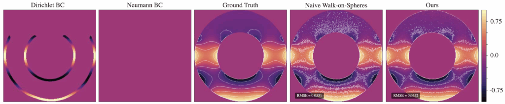
Figure 12. Naive vs. 2-pass method with Dirichlet BC 𝑢 (𝑥, 𝑦) = cos(2𝜋𝑦) and Neumann BC 𝜕𝑢/𝜕𝑛 = 0, num of walks = 128
To handle Neumann boundary conditions, the original WoS algorithm needs to be modified to address the behavior of walks near Neumann boundaries, the radius of closed balls around each point, and conditions for walk termination. The Walk on Stars algorithm (Sawhney et al., 2023) does exactly this. Walk on Stars generalizes WoS by replacing ball-shaped regions with stars — a star being any shape where every boundary point can be “seen” from the centre. At Neumann boundaries, Walk on Stars simulates reflecting Brownian motion — when a walk reaches a Neumann boundary, it is reflected according to the boundary’s normal vector and picks up a contribution of the Neumann condition, \( h \).
Figure 12 illustrates our results with a zero-valued Neumann boundary condition.The 2-pass method still reduces the RMSE compared to Naive WoS with the same number of walks. However, the contours indicate somewhat increased noise near the reflecting boundary compared to the absorbing boundary on our solution.
5.3 Grouping Techniques to Reduce Overfitting and Improve Stability
Figure 13. Density-based grouping, with improved RMSE for Angle Kernel (right)
As detailed in Section 3.3, a major consideration when estimating control variates is the conditioning and placement monopoles. To further address this, we experimented with grouping techniques that compress nearby or similar samples and assign them a shared influence, namely:
Greedy grouping: Choose a point and assign all other points within a fixed radius to one group. Each groups shares either a weight or a single basis function, effectively reducing the number of active degrees of freedom in the system. Our experiments show a reduction in RMSE via grouping for the angle kernel (see Figure 13), but contours indicate a slight increase in noise in some regions.
DBSCAN: This density-based clustering technique automatically identifies dense clusters of points. Each cluster is treated as a group, and only a representative or averaged contribution is retained, while the rest are collapsed into it.
6 Conclusions and Future Directions
We introduced harmonic control variates: a simple, closed-form control variate for Walk-on-Spheres built from mixtures of harmonic kernels. By fitting a lightweight least-squares model once and efficiently evaluating it in closed form during sampling, we turn WoS into a two-pass estimator that remains unbiased while substantially lowering variance. Empirically, our method delivers consistent accuracy gains across diverse geometries—e.g., an average 40% RMSE reduction at 128 walks—while adding only minimal overhead compared to previous neural control variate approaches; as walks dominate runtime, the extra cost is effectively negligible. The result is a method that is easy to implement (a small change to a standard WoS pipeline), robust to geometric complexity, and markedly more sample-efficient.
Future work. We plan to release a plug-in that drops into existing WoS codebases and to continue improving our method for even stronger variance reduction at essentially the same runtime.
References
Jacobson, Alec, Ladislav Kavan, and Olga Sorkine [2013]. “Robust Inside-Outside Segmentation using Generalized Winding Numbers”. In: ACM Trans. Graph. 32.4.
Li, Zilu et al. [2024]. “Neural Control Variates with Automatic Integration”. In: ACM SIGGRAPH 2024 Conference Papers. SIGGRAPH ’24. Denver, CO, USA: Association for Computing Machinery. isbn: 9798400705250. doi: 10.1145/3641519. 3657395. url: https://doi.org/10.1145/3641519.3657395.
Madan, Abhishek et al. [July 2025]. “Stochastic Barnes-Hut Approximation for Fast Summation on the GPU”. In: Proceedings of the Special Interest Group on Computer Graphics and Interactive Techniques Conference Conference Papers. SIGGRAPH Conference Papers ’25. ACM, pp. 1–10. doi: 10.1145/3721238.3730725. url: http://dx.doi.org/10.1145/3721238.3730725.
Muller, Mervin E. [1956]. “Some Continuous Monte Carlo Methods for the Dirichlet Problem”. In: The Annals of Mathematical Statistics 27.3, pp. 569–589. doi: 10.1214/aoms/1177728169. Url: https://doi.org/10.1214/aoms/1177728169.
Nam, Hong Chul, Julius Berner, and Anima Anandkumar [2024]. “Solving Poisson Equations Using Neural Walk-on-Spheres”. In: Forty-first International Conference on Machine Learning
Sawhney, Rohan and Keenan Crane [Aug. 2020]. “Monte Carlo geometry processing: a grid-free approach to PDE-based methods on volumetric domains”. In: ACM Trans. Graph. 39.4. issn: 0730-0301. Doi: 10.1145/3386569.3392374. url: https://doi.org/10.1145/3386569.3392374.
Sawhney, Rohan and Bailey Miller [2023]. Zombie: Grid-Free Monte Carlo Solvers for Partial Differential Equations. Version 1.0.
Sawhney, Rohan, Bailey Miller, et al. [July 2023]. “Walk on Stars: A Grid-Free Monte Carlo Method for PDEs with Neumann Boundary Conditions”. In: ACM Trans. Graph. 42.4. issn: 0730-0301. doi: 10.1145/3592398. url: https://doi.org/10.1145/3592398.
Our work was carried out under the mentorship of Yi Zhuo from Adobe Research, whose guidance was instrumental and very much appreciated. We also thank Sanghyun Son , the first author of the original DMesh and DMesh++ , for generously sharing his insights and providing invaluable input.
Article Composed By: Gabriel Isaac Alonso Serrato in collaboration with Amruth Srivathsan
This article introduces Differentiable Mesh++ (DMesh++), exploring what a mesh is, why discrete mesh connectivity blocks gradient flow, how probabilistic faces restore differentiability, and how a local, GPU-friendly tessellation rule replaces a global weighted Delaunay step. We close with a practical optimization workflow and representative applications.
WHAT IS A MESH?
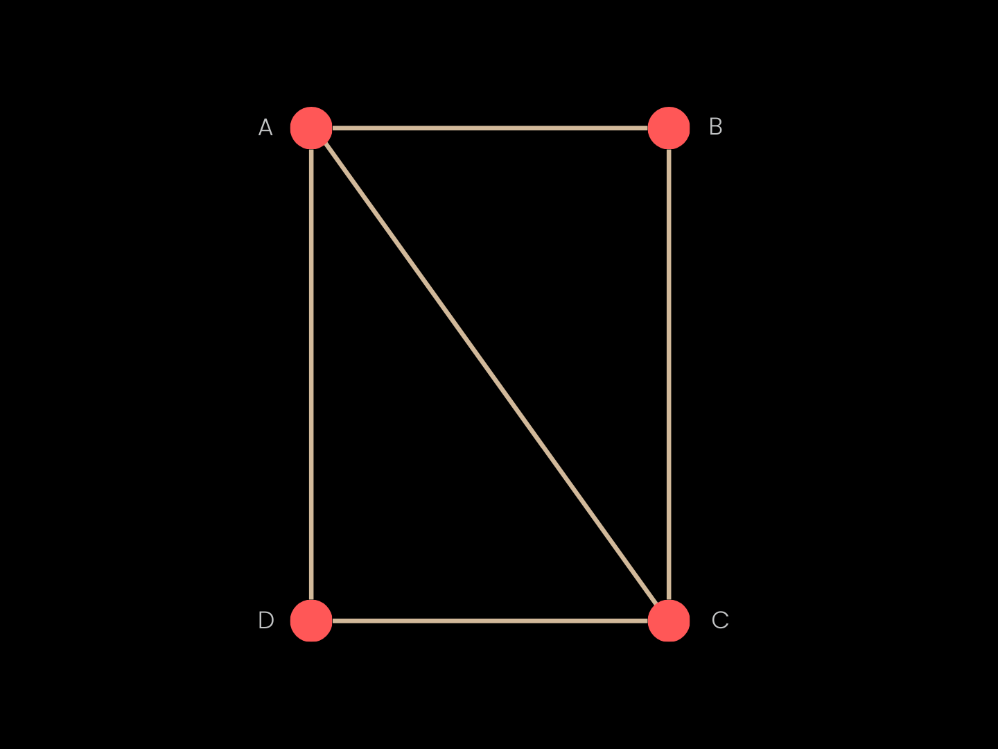
A triangle mesh combines geometry and topology. Geometry is given by vertex coordinates (named points in space such as A, B, C, and D) while topology specifies which vertices are connected by edges and which triplets form triangular faces (e.g., ABC, ACD). Together, these define shape and structure in a compact representation suitable for rendering and computation on complex surfaces.
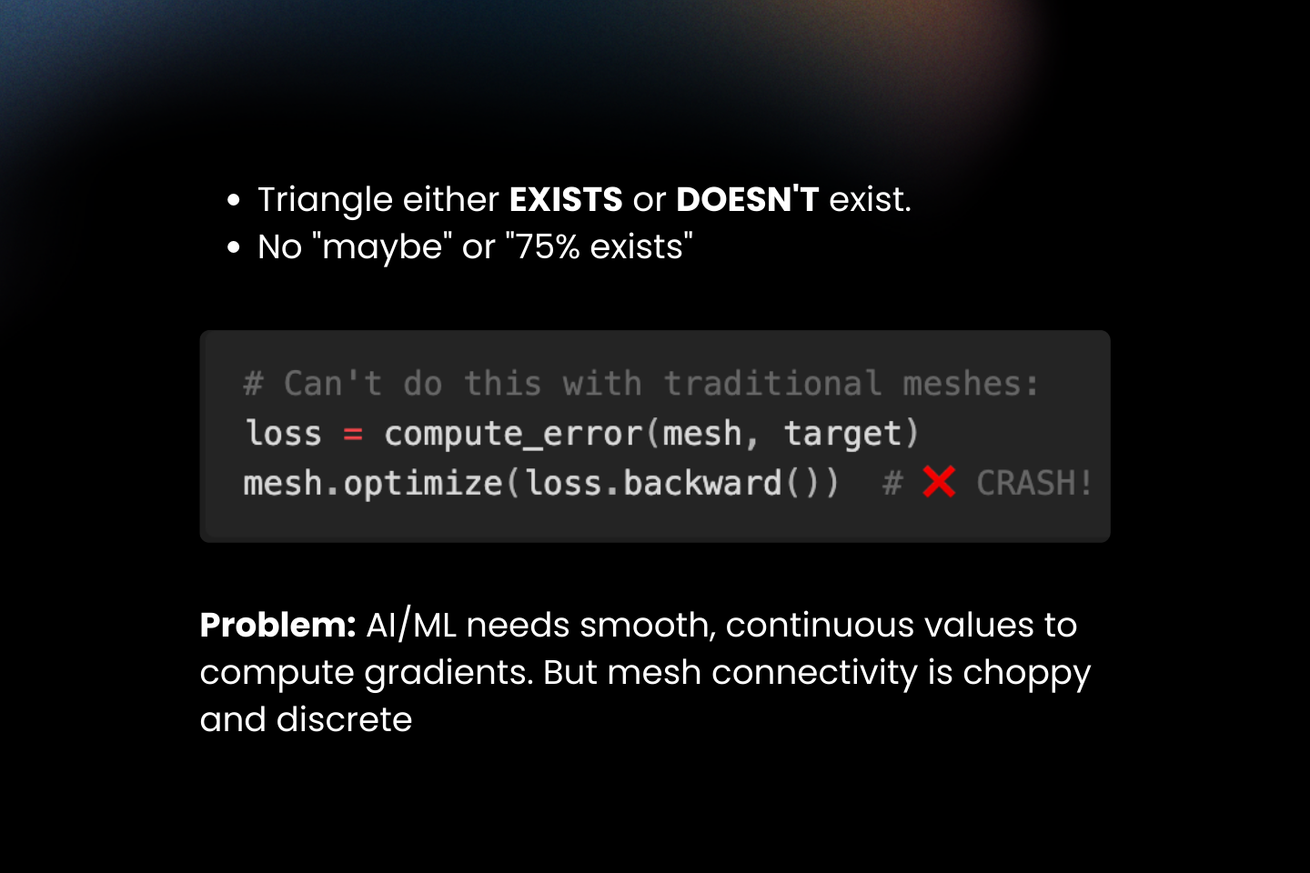
Why Traditional Meshes Fight Gradients?
Classical connectivity is discrete: a triangle either exists or it does not. Gradient-based learning, however, requires smooth changes. When connectivity flips on or off, derivatives vanish or become undefined through those choices, preventing gradients from flowing across topology changes and limiting end-to-end optimization
Differentiable Meshes
Gradients are essential for learning-based pipelines, where losses may be defined in image space, perceptual space, or 3D metric space.
Differentiable formulations make it possible to propagate error signals from rendered observations or physical constraints back to vertex positions, enabling tasks such as inverse rendering, shape optimization, and end-to-end 3D reconstruction. This bridges the conceptual gap between discrete geometry and continuous optimization, allowing mesh-based representations to function as both modeling primitives and trainable structures.
How DMesh++ Works
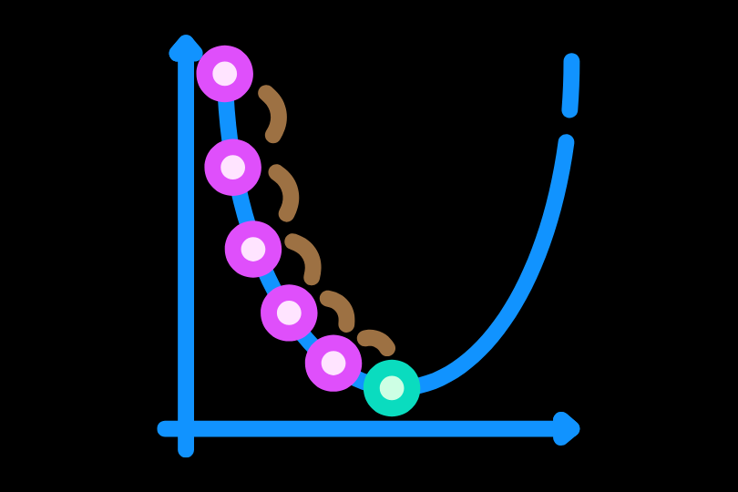
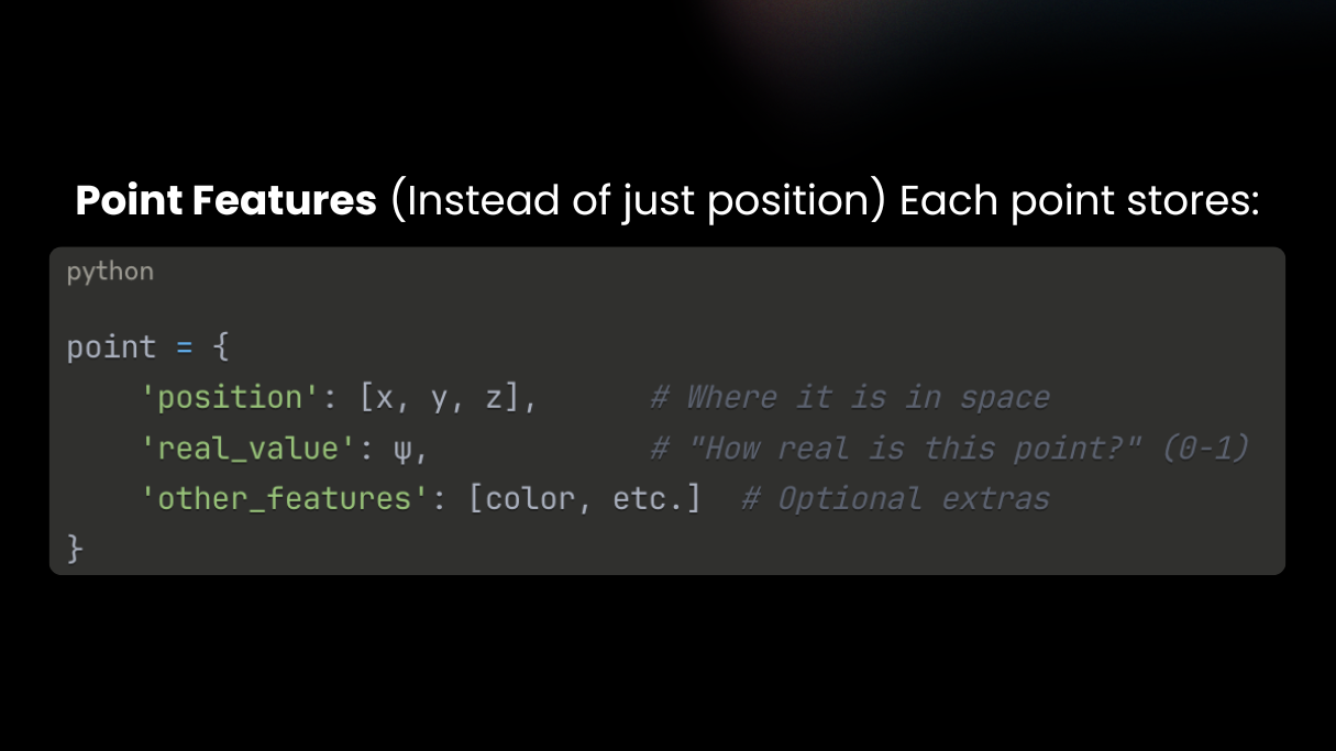
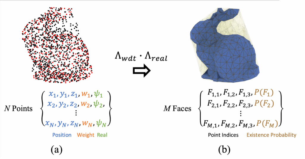
DMesh++ makes meshing a differentiable, GPU-native step. Each point carries learnable features (position, a “realness” score ψ, and optional channels).
A soft tessellation function turns any triplet into a triangle weight rather than a hard on/off face.
During training, losses back-propagate to both positions and features, so connectivity can evolve smoothly.
The “One-Line” Idea in DMesh++
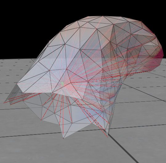
In DMesh++, we replace WDT (Λwdt )
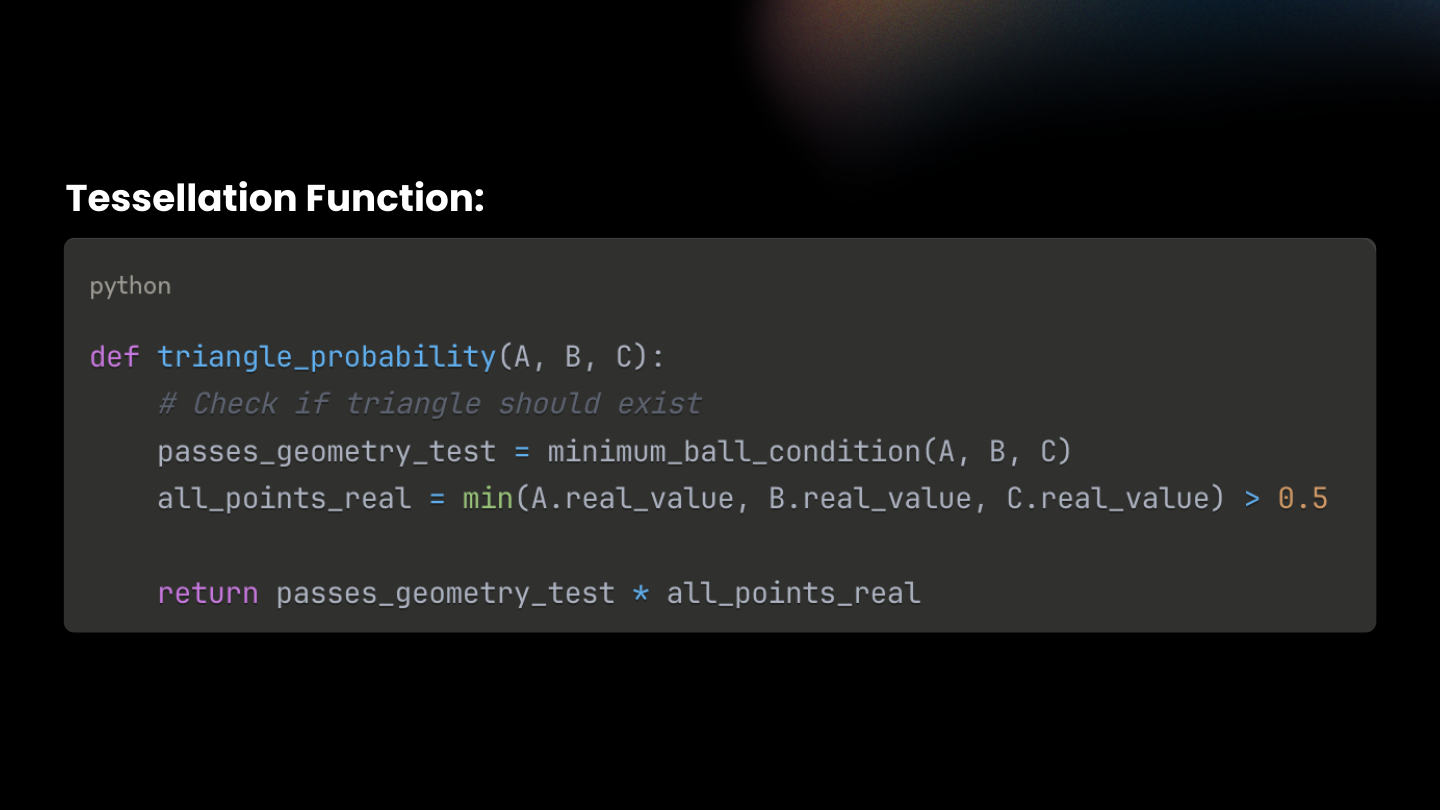
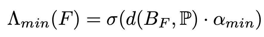
with a local Minimum-Ball test ( Λmin ) when scoring each candidate face. Instead of rebuilding a global structure, we only check the smallest ball touching the face’s vertices and see if any other point lies inside it. This can be done quickly with k-nearest neighbor search on the GPU. The face probability is now:
Λ(F) = Λmin(F) × Λreal(F)
Λmin(F)says, “Is this face even eligible as part of a good tessellation?” (now via the Minimum-Ball test)
Λreal(F) says, “Is this face on the real surface?” (a differentiable min over the per-point realness ψ)
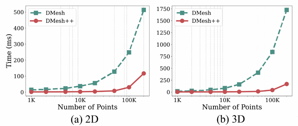
This swap reduces the effective evaluation cost from O(N) (WDT) to O(log N) with k-NN and parallelization, in practice, achieving speeds up to 16× faster in 2D and 32× faster in 3D, with significant memory savings.
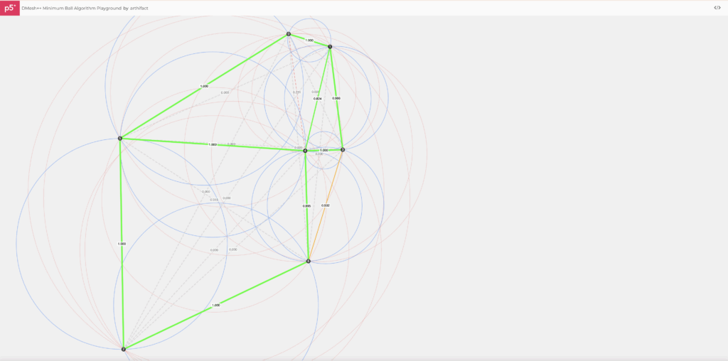
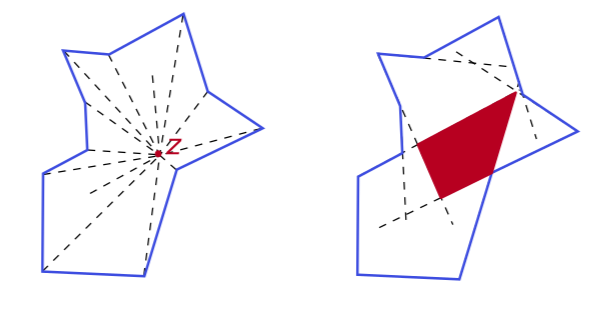
Minimum-Ball, Explained
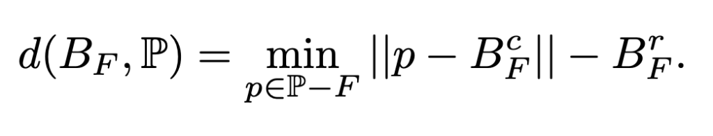
Pick a candidate face F (segment in 2D, triangle in 3D). Compute its minimum bounding ballBF : the smallest ball that touches all vertices of F.
Now check: is any other point strictly inside that ball? If no, F passes. If yes, reject. That’s the Minimum-Ball condition. (It’s a subset of Delaunay, so you inherit good triangle quality and avoid self-intersections.)
DMesh++ makes this soft and differentiable. It computes a signed distance between BF and the nearest other Point and runs it through a sigmoid to get Λmin :
Click on the canvas to drop points. Every pair of points becomes a candidate edge F. We draw the minimum ballBF (the smallest circle touching the two endpoints) and compute a soft eligibility via a sigmoid of its clearance to the nearest third point:
Because faces are probabilistic, the topology can change cleanly during optimization. You don’t hand-edit connectivity; it emerges from the features.
Recap: A Practical Optimization Workflow
Start: Begin with points (positions + realness ψ)
Candidates: Form nearby faces (via k-NN)
Minimum-Ball: For each face, find the smallest ball touching its vertices (if no point is inside, it’s valid) → gives Λₘᵢₙ
Weight by Realness: Multiply by vertex ψ to get final probability Λ = Λₘᵢₙ × Λᵣₑₐₗ
Optimize: Compute the loss (e.g., Chamfer), and backpropagate to update the points and ψ
Output: Keep high-Λ faces → final differentiable mesh
Some Applications of DMesh++
DMesh++ demonstrates how differentiable meshes can power real applications. Here are some ideas:
Generative Design: Train models that evolve shapes and topology for creative or engineering tasks without manual remeshing.
Adaptive Level of Detail: Automatically refine or simplify geometry based on learning signals or rendering needs.
Feature-Aware Reconstruction: Learn geometric structure, merge fragments, or fill missing regions directly through optimization.
Neural Simulation: Enable physics or visual simulations where mesh shape and motion are optimized end-to-end with gradients.
Future Directions
Looking ahead, future work on DMesh++ could focus on improving usability and scalability, for example, by developing more accessible APIs, real-time visualization tools, and integration with common 3D software. On the algorithmic side, enhancing the tessellation functions for higher precision and stability, expanding support for non-manifold and hybrid volumetric surfaces, and further optimizing GPU kernels for large-scale datasets could make differentiable meshing faster, more robust, and easier to adopt across geometry processing, simulation, and machine learning workflows.
SGI Fellows: Haojun Qiu, Nhu Tran, Renan Bomtempo, Shree Singhi and Tiago Trindade Mentors: Sina Nabizadeh and Ishit Mehta SGI Volunteer: Sara Samy
Introduction
The field of Computational Fluid Dynamics (CFD) has long been a cornerstone of both stunning visual effects in movies and video games, and also a critical tool in modern engineering, for designing more efficient cars and aircrafts for example. At the heart of any CFD application there exists a solver that essentially predicts how a fluid moves in space at discrete time intervals. The dynamic behavior of a fluid is governed by a famous set of partial differential equations, called the Navier-Stokes equations, here presented in vector form:
where \(t\) is time, \(\mathbf{u}\) is the varying velocity vector field, \(\rho\) is the fluids density, \(p\) is the pressure field, \(\nu\) is the kinematic viscosity coefficient and \(\mathbf{f}\) represents any external body forces (e.g. gravity, electromagnetic, etc.). Let’s quickly break down what each term means in the first equation, which describes the conservation of momentum:
\(\dfrac{\partial \mathbf{u}}{\partial t}\) is the local acceleration, describing how the velocity of the fluid changes at a fixed point in space.
\((\mathbf{u} \cdot \nabla) \mathbf{u}\) is the advection (or convection) term. It describes how the fluid’s momentum is carried along by its own flow. This non-linear term is the source of most of the complexity and chaotic behavior in fluids, like turbulence.
\(\frac{1}{\rho}\nabla p\) is the pressure gradient. It’s the force that causes fluid to move from areas of high pressure to areas of low pressure.
\(\nu \nabla^{2} \mathbf{u}\) is the viscosity or diffusion term. It accounts for the frictional forces within the fluid that resist flow and tend to smooth out sharp velocity changes. For the “Gaussian Fluids” paper, this term is ignored (\(\nu=0\)) to model an idealized inviscid fluid.
The second equation, \(\nabla \cdot \mathbf{u} = 0\), is the incompressibility constraint. It mathematically states that the fluid is divergence-free, meaning it cannot be compressed or expanded.
The first step to numerically solving these equations on some spatial domain \(\Omega\) using classical solvers is to discretize this domain. To do that, two main approaches have dominated the field from its very beginning:
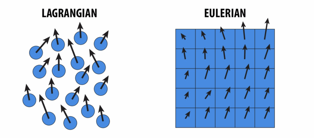
Eulerian methods: which use fixed grids that partition the spatial domain into a (un)structured collection of cells on which the solution is approximated. However, these methods often suffer from “numerical viscosity,” an artificial damping that smooths away fine details;
Lagrangian methods: which use particles to sample the solution at certain points in space and that move with the fluid flow. However, these methods can struggle with accuracy and capturing delicate solution structures.
The core problem has always been a trade-off. Achieving high detail with traditional solvers often requires a massive increase in memory and computational power, hitting the “curse of dimensionality”. Hybrid Lagrangian-Eulerian methods that try to combine the best of both worlds can introduce their own errors when transferring data between grids and particles. The quest has been for a representation that is expressive enough to capture the rich, chaotic nature of fluids without being computationally prohibitive.
A Novel Solution: Gaussian Spatial Representation
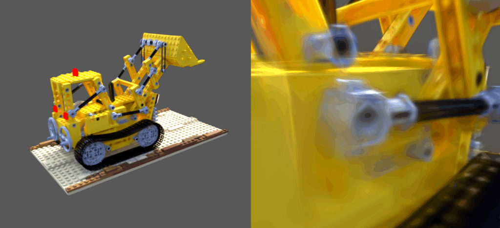
By now you have probably come across an emerging technology in the field of 3D rendering called 3D Gaussian Splatting (3DGS). It attempts to represent a 3D scene using, not traditional polygonal meshes or volumetric voxels, but in a manner similar to an artist using paint brush strokes to approximate a colored picture, Gaussian Splatting uses 3D gaussians to “paint” a 3D scene. These gaussians are nothing more than a ellipsoid with a color value and opacity associated.
Think of each Gaussian not as a solid, hard-edged ellipsoid, but as a soft, semi-transparent cloud (Fig.2). It’s most opaque and dense at its center and it smoothly fades to become more transparent as you move away from the center. The specific shape, size, and orientation of this “cloud” are controlled by its parameters. By blending thousands or even millions of these colored, transparent splats together, Gaussian Splatting can represent incredibly detailed and complex 3D scenes.
Fig.1 Example 3DGS of a Lego build (left) and a zoomed in view of the gaussians that make it up (right).
Drawing from this incredible effectiveness of using gaussians to encode complex geometry and lighting of 3D scenes, a new paper presented at SIGGRAPH 2025 titled “Gaussian Fluids: A Grid-Free Fluid Solver based on Gaussian Spatial Representation” by Jingrui Xing et al. introduces a fascinating new approach to computational domain representation for CFD applications.
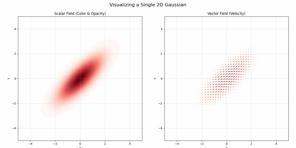
The new method, named Gaussian Spatial Representation (GSR), uses gaussians to essentially “paint” vector fields. While 3DGS encodes local color information into each gaussian, GSR encodes local vector fields. In this way each gaussian stores a vector that defines a local direction of the velocity field, where the magnitude of the vectors is greater closer the gaussian’s center, and quickly gets smaller when moving farther from it. In Fig.2 we can see an example of 2D gaussian viewed with color data (left), as well as with a vector field (right).
Fig.2 Example plot of a 2D Gaussian with scalar data (left) and vector data (right)
By splatting a lot of these gaussians and adding the vectors we can then define a continuously differentiable vector field around a given domain, which allows us to solve the complex Navier-Stokes equations not through traditional discretization, but as a physics-based optimization problem at each time step. A custom loss function ensures the simulation adheres to physical laws like incompressibility (zero-divergence) and, crucially, preserves the swirling motion (vorticity) that gives fluids their character.
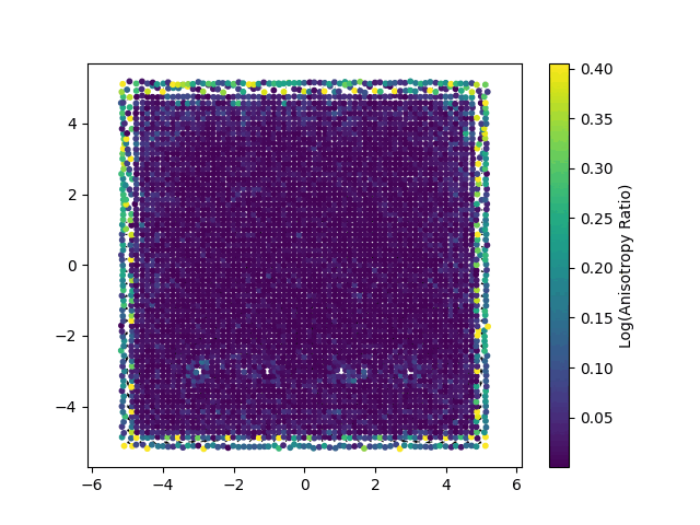
Each point represents a Gaussian splat, with its color mapped to the logarithm of its anisotropy ratio. This visualization highlights how individual Gaussians are stretched or compressed in different regions of the domain.
Enforcing Physics Through Optimization: The Loss Functions
The core of the “Gaussian Fluids” method is its departure from traditional time-stepping schemes. Instead of discretizing the Navier-Stokes equations directly, the authors reframe the temporal evolution of the fluid as an optimization problem. At each time step, the solver seeks to find the set of Gaussian parameters that best satisfies the governing physical laws. This is achieved by minimizing a composite loss function, which is a weighted sum of several terms, each designed to enforce a specific physical principle or ensure numerical stability.
Two of the main loss terms are:
Vorticity Loss (\(L_{vor}\)): For a two dimensional ideal (inviscid) fluid, vorticity, defined as the curl of the velocity field (\(\omega=\nabla \times u\)), is a conserved quantity that is transported with the flow. This loss function is designed to uphold this principle. It quantifies the error between the vorticity of the current velocity field and the target vorticity field, which has been advected from the previous time step. By minimizing this term, the solver actively preserves the rotational and swirling structures within the fluid. This is critical for preventing the numerical dissipation (an artificial smoothing of details) that often plagues grid-based methods and for capturing the fine, filament-like features of turbulent flows.
Divergence Loss (\(L_{div}\)): This term enforces the incompressibility constraint, \(\nabla \cdot u=0\). From a physical standpoint, this condition ensures that the fluid’s density remains constant; it cannot be locally created, destroyed, or compressed. The loss function achieves this by evaluating the divergence of the Gaussian-represented velocity field at numerous sample points and penalizing any non-zero values. Minimizing this term is essential for ensuring the conservation of mass and producing realistic fluid motion.
Beyond these two, to function as a practical solver, the system must also handle interactions with boundaries and maintain stability over long simulations. The following loss terms address these requirements:
Boundary Losses (\(L_{b1}\), \(L_{b2}\)): The behavior of a fluid is critically dependent on its interaction with solid boundaries. These loss terms enforce such conditions. By sampling points on the surfaces of geometries within the scene, the loss function penalizes any fluid velocity that violates the specified boundary conditions. This can include “no-slip” conditions (where the fluid velocity matches the surface velocity, typically zero) or “free-slip” conditions (where the fluid can move tangentially to the surface but not penetrate it). This sampling-based strategy provides an elegant way to handle complex geometries without the need for intricate grid-cutting or meshing procedures.
Regularization Losses (\(L_{pos}\), \(L_{aniso}\), \(L_{vol}\)): These terms are included to ensure the numerical stability and well-posedness of the optimization problem.
The Position Penalty (\(L_{pos}\)) constrains the centers of the Gaussians, preventing them from deviating excessively from the positions predicted by the initial advection step. This regularizes the optimization process, improves temporal coherence, and helps prevent particle clustering.
The Anisotropy (\(L_{aniso}\)) and Volume (\(L_{vol}\)) losses act as geometric constraints on the Gaussian basis functions themselves. They penalize Gaussians that become overly elongated, stretched, or distorted. This is crucial for maintaining a high-quality spatial representation and preventing the numerical instabilities that could arise from ill-conditioned Gaussian kernels.
However, when formulating a fluid simulation as a Physics-Based optimization problem, one challenge that soon becomes apparent is that choosing good loss functions can be really tricky. The reliance on “soft constraints”, such as the divergence loss function, in the optimization process means that small errors can accumulate over time. Also, the handling of complex domains with holes (non-simply connected domains) is also a big challenge. When running the Leapfrog simulation we can see that the divergence of the solution, although relatively small, isn’t as close to zero as it should be (ideally it should be exactly zero).
This “Leapfrog” simulation highlights the challenge of “soft constraints.” The “Divergence” plot (bottom-left) shows the small, non-zero errors that can accumulate, while the “Vorticity” plot (bottom-right) shows the swirling structures the solver aims to preserve.
Divergence-free Gaussian Representation
Now we want to extend on this paper a bit. Let’s focus on the 2D case for now. The problem of regularizing divergence is that the velocity vector field won’t be exactly divergence free. I can perhaps help this with an extra step every iteration. Define \(\mathbf{J} \in \mathbb{R}^{2 \times 2}\) as a rotation matrix
This potential function can be constructed with the same gaussian mixture by carrying a \(\phi_{i} \in \mathbb{R}\) at every gaussian, and thus a continuous function having full support
similarly we can replace \(G_i(\mathbf{x})\) with the clamped gaussians \(\tilde{G}_i(\mathbf{x})\) for efficiency. Now we can construct a vector field that is unconditionally divergence-free
and we use the similar approach of Monte Carlo way of sampling \(\mathbf{x}\) uniformly in space.
Doing this, we managed to achieve a divergence much closer to zero, as shown in the image below.
Before (left) and after (right)
References
Jingrui Xing, Bin Wang, Mengyu Chu, and Baoquan Chen. 2025. Gaussian Fluids: A Grid-Free Fluid Solver based on Gaussian Spatial Representation. In Proceedings of the Special Interest Group on Computer Graphics and Interactive Techniques Conference Conference Papers (SIGGRAPH Conference Papers ’25). Association for Computing Machinery, New York, NY, USA, Article 9, 1–11. https://doi.org/10.1145/3721238.3730620
One of the biggest bottlenecks in the modern model training pipelines for neuroimaging is diverse, well-labeled data. Real clinical MRI scans that could have been used, are under constraints of privacy, scarce annotations, and chaotic protocols. Because open-source MRI data comes from many scanners with different setups, the data varies a lot. This variation causes domain shifts and makes generalization much harder. All of these problems reinforce us to look for other solutions. Synthetic data directly handles these bottlenecks, once we have a robust pipeline that can generate unlimited, labelled data, we can expose models to the full range of scans (contrasts, noise levels, artifacts, orientations). With synthetic data, we are taking a step forward of solving the biggest bottlenecks in model training.
Nevertheless, another important thing is resolution. Most MRI scans are relatively low-resolution. At this scale, thin brain structures blur and different tissues can get mixed in a single voxel, so edges look soft and details disappear. This especially hurts areas like the cortical ribbon, ventricle borders, and small nuclei.
When models are trained only on these blurry data, they learn what they see: oversmoothed segmentations and weak boundary localization. Even with strong architectures and losses, you can’t recover details that simply don’t exist in the initial data that was fed to the model.
We are tackling this problem by generating higher-resolution synthetic data from clean geometric surfaces. Training with these high-resolution, label-accurate volumes gives models a much clearer understanding of what boundaries look like.
From MRI images to Meshes
The generation of synthetic data begins by using an already available brain MRI scan and replicating it into a collection of MRI data such that all the files in this collection represent the same MRI scan. However, each file uses a different set of contrasts to represent different regions of the brain. This ensures that our data collection is representative of the different models of MRI scanning devices available as each device can use a specific set of contrasts different from the ones used by other devices. Furthermore, we can make the orientation of the brain random to allow the data to mimic the randomness of how a person may position their head inside the MRI device. This process can be done easily using the already implemented python tool SynthSeg.
Using SynthSeg
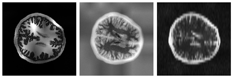
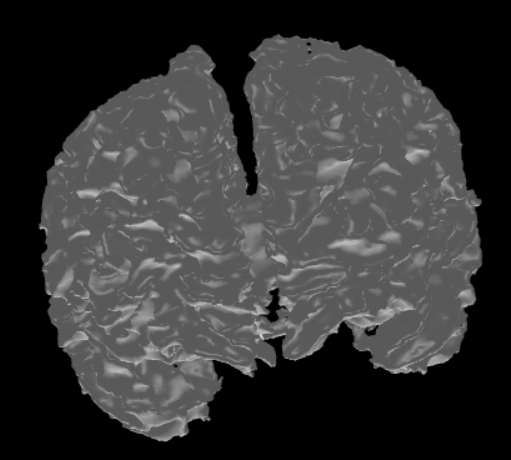
By running the SynthSeg Brain Generator using an available MRI scan, we can get random synthesized MRI data. For illustration, we can generate 3 samples that have different contrasts but the same orientation by setting the number of channels to 3. Here is a cross section of the output of these samples.
The output of the Brain Generator for each instance are two files: an image file and a label file. The image file is an MRI data file that contains all of the scan’s details. On the other hand, the label file is a file that only indicates the boundaries of different structures indicated in the image file.
Mesh Generation
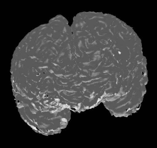
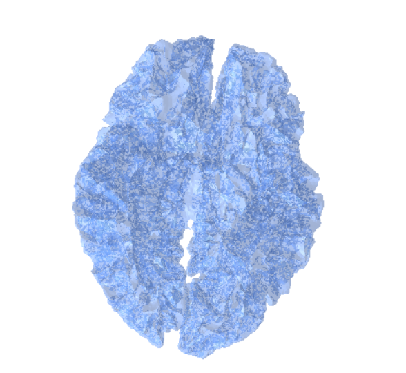
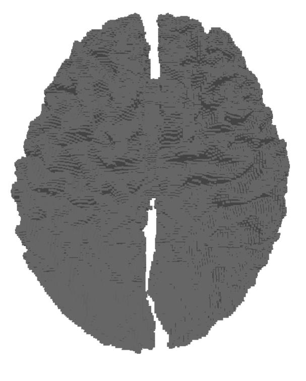
The label files can be useful as they only contain data describing the boundaries of each different region in the MRI data. This makes them more suitable for brain surface mesh generation. Using the SimNIBS package, different meshes can be generated via a label file. Each mesh represents a different region as dictated by the label file. After that, these meshes can be combined together to get a full mesh of the surface of the brain. Here are two meshes generated from the same label file.
From Meshes to MRI Data
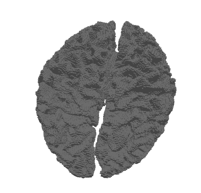
Once the MRI scans are transformed into meshes, the next step is to convert these geometric representations back into volumetric data. This process, called voxelization, allows us to represent the mesh on a regular 3D grid (voxels), which closely resembles the structure of MRI images.
Voxelization Process
Voxelization works by sampling the 3D mesh into a uniform grid, where each voxel stores whether it lies inside or outside the mesh surface. This results in a binary (or occupancy) grid that can later be enriched with additional attributes such as intensity or material properties.
Input: A mesh (constructed from MRI segmentation or surface extraction).
Output: A voxel grid representing the same anatomical structure.
Resolution and Grid Density
The quality of the voxelized data is heavily dependent on the resolution of the grid:
Low-resolution grids are computationally cheaper but may lose fine structural details.
High-resolution grids capture detailed geometry, making them particularly valuable for training machine learning models that require precise anatomical features.
Bridging Mesh and MRI Data
By voxelizing the meshes at higher resolutions than the original MRI scans, we can synthesize volumetric data that goes beyond the limitations of the original acquisition device. This synthetic MRI-like data can then be fed into training pipelines, augmenting the available dataset with enhanced spatial fidelity.
Conclusion
In conclusion, this pipeline can produce high resolution synthetic brain MRI data that can be used for various purposes. The results obtained from this process are representative as the contrasts of the produced MRI data are randomized to mimic the different types of MRI machines. Due to this, the pipeline has the potential to sustain large amounts of data suitable for the training of various models.
Written By
Youssef Ayman
Ualibyek Nurgulan
Daryna Hrybchuk
Special thanks to Dr. Karthik Gopinath for guiding us through this project!
One will probably ask “what is even discrete morse theory?” A good question. But a better question is, “what is even morse theory?”
A Detour to Morse Theory
It would be a sin to not include this picture of a torus on any text for an introduction to Morse Theory.
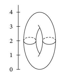
Consider a height function \(f\) defined on this torus \(T\). Let \(M_z = \{x\in T | f(x)\le z\}\), i.e., a slice of the torus below level \(z\).
Morse theory says critical points of \(f\) can tell us something about the topology of the shape. The critical points can be determined by recalling from calculus that those points correspond to the points where the partial derivatives all equal zero. Then, the four critical points on the torus at heights 0, 1, 3, and 4 can be identified, each of which correspond to topological changes in the sublevel sets (\(M_z\)) of the function. In particular, imagine a sequence of sublevel sets \(M_z\) with ever increasing \(z\) values. Notice that each time we pass through a critical point, there is an important topological change in the sublevel sets.
At height 0, everything starts with a point
At height 1, a 1-handle is attached
At height 3, another 1-handle is added
Finally, at height 4, the maximum is reached, and a 2-handle is attached, capping off the top and completing the torus.
Through this process, Morse theory illustrates how the torus is constructed by successively attaching handles, with each critical point indicating a significant topological step.
Discretizing Morse Theory
Originally, Forman introduces discrete Morse Theory to let it inherit many similarities from its smooth counterpart, but it deals with discretized objects like CW complexes or a simplicial complex. In particular, we will focus on discrete morse theory on a simplicial complex.
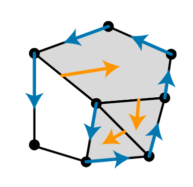
Definition. Let \(K\) be a simplicial complex. A discrete vector field V on \(K\) is a set of pairs of cells \((\sigma, \tau) \in K\times K\), with \(\sigma\) a face of \(\tau\), such that each cell of \(K\) is contained in at most one pair of \(V\). Definition. A cell \(\sigma\in K\) is critical with respect to \(V\) if \(\sigma\) is not contained in any pair of \(V\).
A discrete vector filed V can be readily visualized as a set of arrows like below.
Figure 1. The bottom left vertex is critical
Definition. Let \(V\) be a discrete vector field. A \(V\)-path \(\Gamma\) from a cell \(\sigma_0\) to a cell \(\sigma_r\) is a sequence \((\sigma_0, \tau_0, \sigma_1, \dots, \tau_{r-1}, \sigma_r)\) of cells such that for every \(0\le i\le r-1:\) $$ \sigma_i \text{ is a face of } \tau_i \text{ with } (\sigma_i, \tau_i \in V) \text{ and } \sigma_{i+1} \text{ is a face of } \tau_i \text{ with } (\sigma_{i+1}, \tau_i)\notin V. $$\(\Gamma\) is closed if \(\sigma_0=\sigma_r\), and nontrivial if \(r>0\).
Definition. A discrete vector field V is adiscrete gradient vector field if it contains no nontrivial closed V-paths.
Finally, with this in mind, we can define what properties should a Morse function satisfy on a given simplicial complex \(K\).
Definition. A function \(f: K\rightarrow \mathbb{R}\) on the cells of a complex K is a discrete Morse function if there is a gradient vector field \(V_f\) such that whenever \(\sigma\) is a face of \(\tau\) then $$ (\sigma, \tau)\notin V_f \text{ implies } f(\sigma) < f(\tau) \text{ and } (\sigma, \tau)\in V_f \text{ implies } f(\sigma)\ge f(\tau). $$\(V_f\) is called the gradient vector field of \(f\).
Definition. Let \(V\) be a discrete gradient vector field and consider the relation \(\leftarrow_V\) defined on \(K\) such that whenever \(\sigma\) is a face of \(\tau\) then $$ (\sigma, \tau)\notin V \text{ implies } \sigma\leftarrow_V \tau \text { and } (\sigma, \tau)\in V \text{ implies } \sigma\rightarrow_V \tau. $$ Let \(\prec_V\) be the transitive closure of \(\leftarrow_V\) . Then \(\prec_V\) is called the partial order induced by V.
We are now ready to introduce one of the main theorems of discrete Morse Theory.
Theorem. Let \(V\) be a gradient vector field on \(K\) and let \(\prec\) be a linear extension of \(\prec_{V}\). If \(\rho\) and \(\psi\) are two simplices such that \(\rho \prec \psi\) and there is no critical cell \(\phi\) with respect to \(V\) such that \(\rho\prec\phi\preceq\psi\), then \(\kappa(\psi)\) collapses (homotopy equivalent) to \(\kappa(\rho)\). Here, $$\kappa(\sigma) = closure(\cup_{\rho\in K; \rho\preceq\sigma}\rho)$$ an equivalent of sublevel set in the discrete setting.
This theorem says that given a gradient vector filed to a simplicial complex, and we consider how it is built over time by bringing each simplex in \(\prec\)’s order, then the topological changes happen only at the critical points determined by the gradient vector field. This strikingly is reminiscent of the case with the torus above.
This perspective is not only conceptually elegant but also computationally powerful: by identifying and retaining only the critical simplices, we can drastically reduce the size of our complex while preserving its topology. In fact, several groups of researchers have already utilized the discrete morse theory to simplify a function by removing topological noise.
Reference
Bauer, U., Lange, C., & Wardetzky, M. (2012). Optimal topological simplification of discrete functions on surfaces. Discrete & computational geometry, 47(2), 347-377.
Forman, R. (1998). Morse theory for cell complexes. Advances in mathematics, 134(1), 90-145.
Scoville, N. A. (2019). Discrete Morse Theory. United States: American Mathematical Society.
SGI Fellows: Melisa Oshaini Arukgoda, David Uzor, Lydia Madamopouloua, Joana Owusu-Appiah Mentors: Oliver Gross, Quentin Becker SGI Volunteer: Denisse Garnica
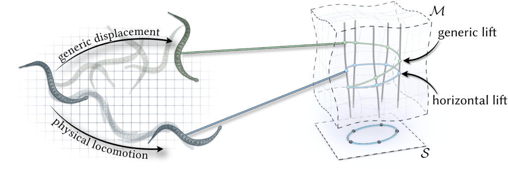
In Week 4 of SGI, we worked on a simulation project that built on the previous work of our Mentors Oliver Gross and Quentin Becker: motion from shape change and inverse geometric locomotion – to put it simply, identifying the sequence of shapes (gait) that a body will need to morph into in order to follow a specific path, without the influence of external forces. In nature, we see this behaviour in many different organisms: Stingrays, snails, Cats (when adjusting their position to allow them to land on their feet after falling), and snakes. Unlike standard physics-based simulations that rely on heavy Newtonian calculations of forces and accelerations, the approach we worked with reformulated the problem as an optimization over shape changes alone. By leveraging conservation laws through geometric mechanics, we could avoid full force-based simulations and instead compute efficient gaits directly — a shift that makes the process both faster and more generalizable.
Motion from Shape Change
Snake-like robots are fascinating because they don’t rely on wheels or legs for movement. Instead, they move by changing their shape over time. This type of motion is called geometric locomotion. By coordinating joint angles in a specific sequence, the robot can “slither” forward, turn, or even back up. Mathematically, we describe this by mapping changes in shape (joint angles) to displacements in space. The beauty of this approach is that the same principles apply whether the robot is operating on flat ground or navigating through more complex environments.
To simulate this, we used Python code that defines the joint angles, applies forward integration, and produces the resulting trajectory. By running sequences of positive and negative angles, we could generate gaits (movement patterns) and measure their effectiveness. Parameters like amplitude, phase shift, and anisotropy ratio all influence how efficient or smooth the motion becomes.
Inverse Geometric Locomotion
While forward motion planning tells us what happens when we execute a gait, inverse geometric locomotion helps us answer the opposite question: what shape sequence do we need to reach a target position or avoid an obstacle? This is formulated as an optimization problem. We define objectives such as “reach this point,” “avoid that obstacle,” or “turn left”, and then optimize the gait until the resulting motion matches the objective.
Here, the gradient descent optimization algorithm is applied to adjust the sequence of joint angles. Our experiments demonstrated that even when constraints are applied (such as broken joints or limited power), the robot can often still achieve meaningful locomotion by adapting its gait.
Breaking and Fixing Robots
One of the challenges with snake robots is robustness. What happens if a joint breaks? We simulated this by disabling certain joints and observing the effect. Unsurprisingly, the robot’s gait efficiency drops, but not all joints are equally important. Some failures severely reduce mobility, while others can be compensated for.
To “fix” the robot, we rerun the optimization process under the new constraints. By adapting the gait, the robot can still move, albeit with reduced performance. This kind of resilience is critical for real-world applications, where hardware failures are inevitable.
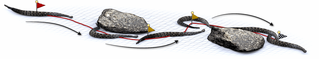
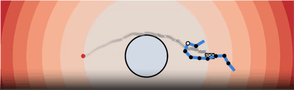
Avoiding Obstacles
Another core part of our experiments was obstacle avoidance. Instead of using explicit geometry, we represented obstacles as implicit functions (mathematical descriptions where the function is positive outside, negative inside, and zero at the boundary). This allows smooth and flexible definitions of obstacles of any shape.
The robot’s motion planner then ensures that the trajectory stays in the safe (positive) region. We tested this with different obstacle shapes and verified that the snake robot can successfully reconfigure its gait to slither around barriers.
Applications
This computational framework for inverse geometric locomotion opens doors for several interesting applications, particularly in the fields of animation and robotics. The video below shows the snake robot in action (courtesy of the MiniRo Lab at the University of Notre Dame), loaded with the shape sequences from the simulation.
SGI Fellows: Lydia Madamopoulou, Nhu Tran, Renan Bomtempo and Tiago Trindade Mentor. Yusuf Sahillioglu SGI Volunteer. Eric Chen
Introduction
In the world of 3D modeling and computational geometry, tackling geometrically complex shapes is a significant challenge. A common and powerful strategy to manage this complexity is to use a “divide-and-conquer” approach, which partitions a complex object into a set of simpler, more manageable sub-shapes. This process, known as shape decomposition, is a classical problem, with convex decomposition and star-shaped decomposition being of particular interest.
The core idea is that many advanced algorithms for tasks like creating volumetric maps or parameterizing a shape are difficult or unreliable on arbitrary models, but work perfectly on simpler shapes like cubes, balls, or star-shaped regions.
The paper by Hinderink et al. (2024) demonstrates this perfectly. It presents a method to create a guaranteed one-to-one (bijective) map between two complex 3D shapes. They achieve this by first decomposing the target shape into a collection of non-overlapping star-shaped pieces. By breaking the hard problem down into a set of simpler mapping problems, they can apply existing, reliable algorithms to each star-shaped part and then stitch the results together. Similarly, the work by Yu & Li (2011) uses star decomposition as a prerequisite for applications like shape matching and morphing, highlighting that star-shaped regions have beneficial properties for many graphics tasks.
Ultimately, these decomposition techniques are a foundational tool, allowing researchers and engineers to extend the reach of powerful geometric algorithms to handle virtually any shape, no matter how complex its structure. Some applications include:
Guarding and Visibility Problems. Star decomposition is closely related to the 3D guarding problem: how can you place the fewest number of sensors or cameras inside a space so that every point is visible from at least one of them? Each star-shaped region corresponds to the visibility range of a single guard. This is widely used in security systems, robot navigation and coverage planning for drones.
Texture mapping and material Design. Star decomposition makes surface parameterization much easier. Since each region is guaranteed to be visible from a point, its much simpler to unwrap textures (like UV mapping), apply seamless materials and paint and label parts of a model.
Fabrication and 3D printing. When preparing a shape for fabrication, star decomposition helps with designing parts for assembly, splitting objects into printable segments to avoid overhangs. It’s particularly useful for automated slicing, CNC machining, and even origami-based folding of materials.
Shape Matching and Retrieval. As mentioned in Hinderink et al. (2024), matching or searching for shapes based on parts is a common task. Star decomposition provides a way to extract consistent, descriptive parts, enabling sketch-based search, feature extraction for machine learning, and comparison of similar objects in 3D data sets.
In this project, we tackle the problem of segmenting a mesh into star-shaped regions. To do this, we explore two different approaches to try to solve this problem:
An interior based approach, where we use interior points on the mesh to create the mesh segments;
A surface based approach, where we try to build the mesh segments by using only surface information.
We then discuss results and challenges of each approach.
What is a star-shape?
You are probably familiar with the concept of a convex shape, that is a shape such that any two points on inside or on the boundary can be connected by straight line without leaving the shape. In simpler terms we can say that a shape is convex if any point inside it has a direct line of sight to any other point on its surface.
Now a shape is called star-shaped if there’s at least one point inside it from which you can see the entire object. Think of it like a single guard standing inside a room; if there’s a spot where the guard can see every single point on every wall without their view being blocked by another part of the room, then the room is star-shaped. This point is called a kernel point, and the set of all possible points where the guard could stand is called the shape’s visibility kernel. If this kernel is not empty, the shape is star-shaped.
On the left we see an irregular non-convex closed polygon where a kernel point is shown along with the lines that connect it to all other vertices.
On the right we now show its visibility kernel in red, that is the set of all kernel points. Also, it is important to note that the kernel may be computed by simply taking the intersection of all inner half-planes defined by each face, i.e. the half-planes of each face whose normal vector points to the inside of the shape.
As a 3D example, we shown in the image bellow a 3D mesh of the tip of a thumb, where we can see a green point inside the mesh (a kernel point) from which red lines are drawn to every vertex of the mesh.
3D mesh example showing a kernel point.
Point Sampling
Before we explore the 2 approaches (interior and surface), we first go about finding sample points on the mesh from which to grow the regions. These can be both interior and surface points.
Surface points
To sample points on a 3D surface, several strategies exist, each with distinct advantages. The most common approaches are:
Uniform Sampling: This is the most straightforward method, aiming to distribute points evenly across the surface area of the mesh. It typically works by selecting points randomly, with the probability of selection being proportional to the area of the mesh’s faces. While simple and unbiased, this approach is “blind” to the actual geometry, meaning it can easily miss small but important features like sharp corners or fine details.
Curvature Sampling: This is a more intelligent, adaptive approach that focuses on capturing a shape’s most defining characteristics. The core idea is to sample more densely in regions of high geometric complexity. These areas, often called “interest points,” are identified by their high curvature values, such as Gaussian curvature (\(\kappa_G\)) or mean curvature (\(\kappa_H\)). By prioritizing these salient features (corners, edges, and sharp curves), this method produces a highly descriptive set of sample points that is ideal for creating robust shape descriptors for matching and analysis.
Farthest-Point Sampling (FPS): This iterative algorithm is designed to produce a set of sample points that are maximally spread out across the entire surface. The process is as follows:
A single starting point is chosen randomly.
The next point selected is the one on the mesh that has the greatest geodesic distance (the shortest path along the surface) to the first point.
Each subsequent point is chosen to be the one farthest from the set of all previously selected points.
This process is repeated until the desired number of samples is reached.
In this project we implemented the curvature and FPS methods. However, none of these approaches gave us the desired distribution of points. So we came up with a hybrid approach: Farthest-Point Curvature-Informed sampling (FPCIS) . It aims to achieve a balance between two competing goals:
Coverage: The sampled points should be spread out evenly across the entire surface, avoiding large unsampled gaps. This is the goal of the standard Farthest Point Sampling (FPS) algorithm.
Feature-Awareness: The sampled points should be located at or near geometrically significant features, such as sharp edges, corners, or deep indentations. This is where curvature comes into play.
We start by selecting the highest curvature point in the mesh. Then, similar to FPS we compute the geodesic distances from this selected point to all other points using the Dijkstra algorithm over the mesh. However, instead of just taking the farthest point, we first create a pool of the top 30% farthest points, and from this pool we then select the one with highest curvature. The subsequent points are chosen in a similar manner to FPS.
Visualization of surface point sampling methods created using Polyscope.
The image above shows the sampling of 15 points using pure FPS (left) and using the FPCIS (right). we see that although FPS gives a pretty well distributed set of sample points we found that some regions that we deemed important where being left out. For example, when sampling 15 points using FPS on the cat model one of the ears was not being sampled. When using the curvature-informed approach we can see that the important regions are correctly sampled.
Interior points
To achieve a list of points that lie well inside the mesh and have good visibility out to the surface, we cast rays inward from every face and recording where they first hit the opposite side of the mesh. Concretely:
For each triangular face, we compute its centroid.
We flip the standard outward face normal to get an inward direction \(d\).
From each centroid, we cast a ray along \(d\), offset by a tiny \(\epsilon\) so it doesn’t immediately self‐intersect.
We use the Möller–Trumbore algorithm to find the first triangle hit by each ray.
The midpoint between the ray origin and its first intersection point becomes one of our skeletal nodes—a candidate interior sample.
Casting one ray per face can produce thousands of skeletal nodes. We apply two complementary down‐sampling techniques to reduce this to a few dozen well‐distributed guards:
EuclideanFarthest Point Sampling (FPS)
Start from an arbitrary seed node.
Iteratively pick the next node that maximizes the minimum Euclidean distance to all previously selected samples.
This spreads points evenly over the interior “skeleton” of the mesh.
k-Means Clustering
Cluster all the midpoints into k groups via standard k-means in \(\mathbb R^3\).
Use each cluster centroid as a down‐sampled guard point.
This tends to place more guards in densely populated skeleton regions while still covering sparser areas.
Interior Approach
Building upon the interior points sampled earlier, Yu & Li (2011) proposed 2 methods to decompose the mesh into star-shaped pieces: Greedy and Optimal.
1. Greedy Strategy
To achieve this, we solve a fast set-cover heuristic:
Repeatedly pick the guard whose visible-face set covers the most currently uncovered faces, remove those faces, and repeat until every face is covered.
For each guard \(g\), we shoot one ray per face-centroid to decide which faces it can “see.” We store these as sets $$ C_j=\{i: \text{face i is visible from } g_j\}$$
Let \(U = { 0,1,…, |F|−1}\) be the set of all uncovered faces.
Repeat the following steps until \(U\) is empty:
For each guard j, compute the number of new faces it would cover: $$ s_j = | C_j \cap U | $$
Pick the guard j with the largest \(s_j\).
Record one star-patch of size \(s_j\).
Remove those faces: \(U = U \backslash C_j\).
Output: Get a list of guard indices (= number of star-shaped pieces) that covers the entire mesh.
2. Optimal Strategy
To get the fewest possible star-pieces from the pre-determined finite set of candidate guards, we cast the problem exactly as a minimum set-cover integer program:
Decision variables: Introduce binary \(x_j \in \{0,1\}\) for each guard \(g_j\).
Every face i must be covered by at least one selected guard (constraint) and we aim to minimize the total number of guards (thus pieces), hence together we solve:
The overall pipeline of our implementation is as follows:
We build the \(|F| \times L\) visibility matrix in sparse COO format.
We feed it to SciPy’s milp, wrapping the “≥1” rows in a LinearConstraint and all variables as binary in a single Bounds object.
The solver returns the provably optimal set of \(x_j\). The optimization problem can be stated as \(\min \sum_{i=1}^m x_i\) subject to \(x_i=0,1\) and \(\sum_{j\in J(i)} x_j\ge 1, \forall i\in\{1,\dots,n\}\).
Experimental Results
We ran both methods on a human hand mesh with 1515 vertices and 3026 faces. The results are shown below:
Results from Greedy algorithm (left) and Optimal ILP solver (right)
Down-sampling method
Strategy
# of candidate guards
# of star-shaped pieces
Piece connectivity
FPS sampling
Greedy
25
13
No
50
9
Yes
Optimal
25
9
No
50
6
No
K-means clustering
Greedy
25
8
No
50
8
No
Optimal
25
7
No
50
6
No
Some key observations are:
Both interior approaches have no constraints to ensure connectivity among faces of the same guard, hence causing difficulties in closing the mesh of each piece or inaccurate calculation of final connected piece number.
Down-sampling methods: k‐means clustering tends to slightly better distribute guards in high‐density skeleton regions, hence having a smaller gap between greedy and optimal strategy.
Surface Approach: Surface-Guided Growth with Mesh Closure
One surface-based strategy we explored is a region-growing method guided by local surface connectivity and kernel validation, with explicit mesh closure at each step. The goal is to grow star-shaped regions from sampled points, ensuring at every expansion that the region remains visible from at least one interior point.
This method operates in parallel for each of the N sampled seed points. Each seed initiates its own region and grows iteratively by considering adjacent faces.
Expansion Process
Initialization:
Begin with the seed vertex and its immediate 1-ring neighborhood—i.e., the three faces incident to the sampled point.
Iterative Expansion:
Identify all candidate faces adjacent to the current region (i.e., faces sharing an edge with the region boundary).
Sort candidates by distance to the original seed point.
For each candidate face:
Temporarily add the face to the region.
Close the region to form a watertight patch using one of the following mesh-closing strategies:
Centroid Fan – Connect boundary vertices to their centroid to create triangles.
2D Projection + Delaunay – Project the boundary to a plane and apply a Delaunay triangulation.
Run a kernel visibility check: determine if there exists a point (the kernel) from which all faces in the current region + patch are visible.
If the check passes, accept the face and continue.
If not, discard the face and try the next closest candidate.
If no valid candidates remain, finalize the region and stop its expansion.
Results and Conclusions
The kernel check was not robust enough—some regions were allowed to grow into areas that clearly violated visibility constraints.
Region boundaries could expand too aggressively, reaching parts of the mesh that shouldn’t logically belong to the same star-shaped segment.
Small errors in patch construction led to instability in the visibility test, particularly for thin or highly curved regions.
As such, the final segmentations were often overextended or incoherent, failing to produce clean, usable star regions. Despite these issues, this approach remains a useful prototype for purely surface-based decomposition, offering a baseline for future improvements in kernel validation and mesh closure strategies.
Expansion with the acquired region at the step.
Expansion step showing mesh and its closing patch.
References
Steffen Hinderink, Hendrik Brückler, and Marcel Campen. (2024). Bijective Volumetric Mapping via Star Decomposition. ACM Trans. Graph. 43, 6, Article 168 (December 2024), 11 pages. https://doi.org/10.1145/3687950
Project Mentors: Sainan Liu, Ilke Demir and Alexey Soupikov
Volunteer Assistant: Vivien van Veldhuizen
Introduction
What is Gaussian Splatting?
3D Gaussian Splatting (3DGS) is a new technique for scene reconstruction and rendering. Introduced in 2023 (Kerbl et al., 2023), it sits in the same family of methods as Neural Radiance Fields (NeRFs) and point clouds, but introduces key innovations that make it both faster and more visually compelling.
To better understand where Gaussian Splatting fits in, let’s take a quick look at how traditional 3D rendering works. For decades, the standard approach to building 3D scenes has relied on mesh modelling — a representation built from vertices, edges, and faces that form geometric surfaces. These meshes are incredibly flexible and are used in everything from video games to 3D printing. However, mesh-based pipelines can be computationally intensive to render and are not ideal for reconstructing scenes directly from real-world imagery, especially when the geometry is complex or partially occluded.
This is where Gaussian Splatting comes in. Instead of relying on rigid mesh geometry, it represents scenes using a cloud of 3D Gaussians — small, volumetric blobs that each carry position, color, opacity, and orientation. These Gaussians are optimized directly from multiple 2D images and then splatted (projected) onto the image plane during rendering. The result is a smooth, continuous representation that can be rendered extremely fast and often looks more natural than mesh reconstructions. It’s particularly well-suited for real-time applications, free-viewpoint rendering, and artistic manipulation, which makes it a perfect match for style transfer, as we’ll see next.
What is Style Transfer?
Figure 1: 2D Style Transfer via Neural Algorithm (Gatys et al., 2015)
Style transfer is a technique in computer vision and graphics that allows us to reimagine a given image (or in our case, a 3D scene) by applying the visual characteristics of another image, known as the style reference. In its most familiar form, style transfer is used to turn photos into “paintings” in the style of artists like Van Gogh or Picasso, as seen in Figure 1. This is typically done by separating the content and style components of an image using deep neural networks, and then recombining them into a new, stylized output.
Traditionally, style transfer has been limited to 2D images, where convolutional neural networks (CNNs) learn to encode texture, color, and brushstroke patterns. But extending this to 3D representations — especially ones that support free-viewpoint rendering — has remained a challenge. How do you preserve spatial consistency, depth, and lighting, while also injecting artistic style?
This is exactly the challenge we’re exploring in our project: applying style transfer to 3D scenes represented with Gaussian Splatting. Unlike meshes or voxels, Gaussians are inherently fuzzy, continuous, and rich in appearance attributes, making them a surprisingly flexible canvas for artistic manipulation. By modifying their colors, densities, or even shapes based on style references, we aim for new forms of stylized 3D content — imagine dreamy impressionist cityscapes or comic-book-like architectural walkthroughs. While achieving consistent and efficient rendering in all cases remains an open challenge, Gaussian Splatting offers a promising foundation for exploring artistic control in 3D.
We present a brief comparison of StyleGaussian and ABC-GS baselines, aiming to extend to style transfer for dynamic patterns, 4D scenes, and localized regions of 3DGS.
Style Gaussian Method
The StyleGaussian pipeline (Liu et al., 2024) achieves stylized rendering of Gaussians with real-time rendering and multi-view consistency through three key steps for style transfer: embedding, transfer, and decoding.
Step 1: Feature Embedding Given a Gaussian Splat and camera positions, the first stage of stylization is embedding deep visual features into the Gaussians. To do this, StyleGaussian uses VGG, a classical CNN architecture trained for image classification. Specifically, features are extracted from the ReLU3_1 layer, which captures mid-level textures like edges and contours that are useful for stylization. These are called VGG features, and they act like high-level visual descriptors of the content of an image. However, VGG features are high-dimensional (256 channels or more), and trying to render them directly through Gaussian Splatting might overwhelm the GPU.
Figure 2: Transformations for Efficient Feature Embedding (Liu et al., 2024)
To solve this, StyleGaussian uses a clever two-step trick illustrated in Figure 2. Instead of rendering all 256 dimensions at once, the program first renders a compressed 32-dimensional feature representation, shown as F’ in the diagram. Then, it applies an affine transformation T to map those low-dimensional features back up to full VGG features F. This transformation can either be done at the level of pixels (i) or at the level of individual Gaussians (ii) — in either case, we recover high-quality feature embeddings for each Gaussian using much less memory.
During training, the system aims to minimize the difference between predicted and true VGG features, so that each Gaussian carries a compact and style-aware feature representation, ready for stylization in the next step.
Step 2: Style Transfer With VGG features embedded, the next step is to apply the style reference. This is done using a fast, training-free method called AdaIN (Adaptive Instance Normalization). AdaIN works by shifting the mean and variance of the feature vectors for each Gaussian so that they match those of the reference image, “repainting” the features without changing their structure. Since this step is training-free, StyleGaussian can apply any new style in real time.
Figure 3: Sample Style Transfer (style references provided by StyleGaussian)
Step 3: RGB Decoding After the style is applied, each Gaussian now carries a modified feature vector — a set of abstract values the neural network uses to describe patterns like brightness, curvature, textures, etc. To render the image, this feature vector needs to be converted into RGB colors for each Gaussian. StyleGaussian does this via a 3D CNN that operates across neighboring Gaussians. This network is trained using a small subset of the style reference images. By comparing a rendered view of the style-transfer to the reference, the network learns how to color the entire scene in a way that reflects the chosen artistic style.
ABC-GS Method
While StyleGaussian offers impressive real-time stylization using feature embeddings and AdaIN, it has a major limitation: it treats the entire scene as a single unit. That means the style is applied uniformly across the whole 3D reconstruction, with no understanding of different objects or regions within the scene.
This is where ABC-GS (Alignment-Based Controllable Style Transfer for 3D Gaussian Splatting) brings something new to the table.
Rather than applying style globally, ABC-GS (Liu et al., 2025) introduces controllability and region-specific styling, enabling three distinct modes of operation:
Single-image style transfer: Apply the visual style of a single image uniformly across the 3D scene, similar to traditional style transfer.
Compositional style transfer: Blend multiple style images, each assigned to a different region of the scene. These regions are defined by manual or automatic masks on the content images (e.g., using SAM or custom annotation). For example, one style image can be applied to the sky, another to buildings, and a third to the ground — each with independent control.
Semantic-aware style transfer: Use a single style image that contains multiple internal styles or textures. You extract distinct regions from this style image (e.g., clouds, grass, brushstrokes) and assign them to matching parts of the scene (e.g., sky, ground) via semantic masks of the content. These masks can be generated automatically (with SAM) or refined manually. This allows for highly detailed region-to-region alignment even within one image.
Figure 4: ABC-GS Single Image Style Transfer
The Two-Stage Stylization Pipeline
ABC-GS achieves stylization using a two-stage pipeline:
Stage 1: Controllable Matching Stage (used in modes 2 and 3 only) In compositional and semantic-aware modes, this stage prepares the scene for region-based style transfer. It includes:
Mask projection: Content and style masks are projected onto the 3D Gaussians.
Style isolation: Each region of the style image is isolated to avoid texture leakage.
Color matching: A linear color transform aligns the base colors of each content region with its assigned style region.
This stage is not used in the single-image mode, since the entire scene is styled uniformly without regional separation.
Stage 2: Stylization Stage (used in all modes) In all three modes, the scene undergoes optimization using the FAST loss (Feature Alignment Style Transfer). This loss improves upon older methods like NNFM by aligning entire distributions of features between the style image and the rendered scene. It captures global patterns such as brushstroke directions, color palette balance, and texture consistency – even in single-image style transfer, FAST consistently yields more coherent and faithful results.
To preserve geometry and content, the stylization is further regularized with:
Content loss: Retains original image features.
Depth loss: Maintains 3D structure.
Regularization terms: Prevent artifacts like over-smoothed or needle-like Gaussians.
Together, these stages make ABC-GS uniquely capable of delivering stylized 3D scenes that are both artistically expressive and structurally accurate — with fine-grained control over what gets stylized and how.
Visual & Quantitative Comparison
Figure 5 illustrates style transfer applied to a truck composed of approximately 300k Gaussians by StyleGaussian (left) and ABC-GS (right). In choosing simple patterns like a checkerboard or curved lines, we hope to highlight how each method handles the key challenges of 3D style transfer, such as alignment with underlying geometry, multi-view consistency, and accurate pattern representation.
To evaluate these differences from a quantitative angle, Fréchet Inception Distance (FID) and Learned Perceptual Image Patch Similarity (LPIPS) metrics were used.
FID measures the distance between the feature distributions of two images sets, with lower scores indicating greater similarity. This metric is often used in generative adversarial network (GAN) and neural style transfer research to assess how well generated images match a target domain. Meanwhile, LPIPS measures perceptual similarity between image pairs by comparing deep features from a pre-trained network, with lower scores indicating better content preservation.
For our purposes, FID measures style fidelity (how well stylized images match the style reference), with scores generally between 0 and 200, and lower scores indicating strong style similarity. LPIPS measures geometry and content preservation (how well the original scene structure is retained) within a range [0, 1], with lower scores indicating better structural preservation.
Figure 5: Comparison between StyleGaussian and ABC-GS
There is a clear visual improvement in the geometric alignment of patterns in the ABC-GS style transfer, where patterns adhere more cleanly with the object boundaries. In contrast, StyleGaussian shows a more diffuse application, with some color-bleeding and areas with high pattern variance (e.g., the wooden panels on the truck). In terms of LPIPS and FID scores, ABC-GS generally outperforms StyleGaussian, but tends to apply a less stylistically-accurate transfer with regular patterns (i) compared to more “abstract” ones (iii).
This difference in performance may stem from how StyleGaussian and ABC-GS handle feature alignment and geometry preservation. StyleGaussian applies a zero-shot AdaIN shift to all Gaussians, matching only the mean and variance of features; since higher-order structure is ignored, patterns can drift onto the wrong parts of the geometry. In contrast, ABC-GS optimizes the scene via FAST loss, computing a transformation that aligns the entire feature distribution of the rendered scene to that of the style. Meanwhile, content loss keeps the scene recognizable, depth loss maintains 3D geometry, and Gaussian regularization prevents distortions, resulting in better LPIPS and FID scores overall. However, in a case like (ii) where there is a lot of white background, ABC-GS’s competing content, depth, and regularization losses prevent large areas to be overwritten with pure white. Instead, it will try to keep more of the original scene’s detail and contrast, especially around geometry edges, which causes a deviation from the style reference and higher FID score. This interplay between geometry and style preservation is a key tradeoff in style transfer.
Although FID and LPIPS metrics are well-established in 2D image synthesis and style transfer, it is important to recognize potential limitations of applying them directly to 3D style transfer. These metrics operate on individual rendered views, without considering multi-view consistency, depth alignment, or temporal coherence. Future works should aim to better understand these benchmarks for 3D scenes.
Extensions & Experiments
Localized Style Transfer: Unsupervised Structural Decomposition of a LEGO Bulldozer via Gaussian Splat Clustering
We explore a novel technique for structural decomposition of complex 3D objects using the latent feature space of Gaussian Splatting. Rather than relying on pre-defined semantic labels or handcrafted segmentation heuristics, we directly use the parameters of a trained Gaussian Splat model as a feature embedding for clustering.
Motivation
The aim was twofold:
Discovery – to see whether clustering Gaussians reveals structural groupings that are not immediately obvious from the visual appearance.
Applicability – to explore whether these groupings could be useful for style transfer workflows, where distinct regions of a 3D object might be stylized differently based on structural identity.
Method
We trained a Gaussian Splatting model on a multi-view dataset of a LEGO bulldozer. The model was optimized to reconstruct the object from multiple angles, producing a 3D representation composed of thousands of oriented Gaussians.
From this representation, we extracted the following features per Gaussian:
3D Position(x, y, z) (weighted for stronger spatial influence)
Color(r, g, b)
Scale(scale_0, scale_1, scale_2) (downweighted to avoid overemphasis)
Opacity(if available)
Normal Vector(nx, ny, nz)(surface orientation)
These features were concatenated into a single vector per Gaussian, weighted appropriately, and standardized. We applied KMeans clustering to segment the Gaussian set into six groups.
Results
The clustering revealed six distinct regions within the bulldozer’s Gaussian representation, each with unique spatial, chromatic, and geometric signatures.
Figure 6: Statistics for 6 Clusters
Figure 7: Visualization of KMeans groupings
Conclusion
The clustering was able to segment the bulldozer into regions that loosely align with intuitive sub-parts (e.g., the bucket, cabin, and rear assembly), but also revealed less obvious groupings—particularly in areas with subtle differences in surface orientation and scale that are hard to distinguish visually. This suggests that Gaussian-parameter-based clustering could serve as a powerful tool for automated part segmentation without requiring labeled data.
Future Work
Cluster Refinement – Experiment with different weighting schemes and feature subsets (e.g., excluding normals or opacity) to evaluate their effect on segmentation granularity.
Hierarchical Clustering – Apply multi-level clustering to capture both coarse and fine structural groupings.
Style Transfer Applications – Use cluster assignments to drive localized style transformations, such as recoloring or geometric exaggeration, to test their value in content creation workflows.
Cross-Object Comparison – Compare clustering patterns across different models to see if similar structural motifs emerge.
Dynamic Texture Style Transfer
Next, given StyleGaussian’s ability to apply new style references at runtime, a natural extension is style transfer of dynamic patterns. Below are some initial results of this approach, created by cycling through the frames of a gif or video in predetermined time intervals.
There is a key tradeoff between flexibility and quality: while zero-shot transfer enables dynamic patterns, the features are relatively muddled, making it difficult to project detailed media. Meanwhile, in the case of ABC-GS, this improved stylization is a result of optimization, which cannot occur at runtime as with StyleGaussian, making it difficult to render dynamic patterns.
Dynamic Scene Style Transfer
So far we’ve shown how incredibly powerful 3D Gaussian Splatting (3DGS) is for generating 3D static scene representations with remarkable detail and efficiency. The parallel to the dawn of photography is a compelling one: just as early cameras first captured the world on a static 2D canvas, 3DGS excels at creating photorealistic representations of real world scenes on a static 3D canvas. A logical next step is to leverage this technology to capture dynamic scenes.
Videos represent dynamic 2D scenes by capturing a series of static images that, when shown in rapid succession, let us perceive subtle changes as motion. In a similar fashion, one may attempt to capture dynamic 3D scenes as a sequence of static 3D scene representations. However, the curse of dimensionality plagues any naive approach to bring this idea to reality.
Lessons from Video Compression
In the digital age of motion picture, storing a video naively as a sequence of individual images (imitating a physical film strip) is possible but hugely inefficient. A digital image is nothing more than a 2D grid of small elements called pixels. In most image formats, each pixel usually stores about 3 bytes of color data, and a good quality Full HD image contains around 1920 x 1080 ≈ 2 million pixels. This amounts to around 6 million bytes (6 MB) of memory needed to store a single uncompressed Full HD image. Now, a reasonably good video should capture 1 second of a dynamic scene using 24 individual images (24 fps), which yields 144 MB of data to capture just a single second of uncompressed video (using uncompressed images). This means that a quick 30-second video would require a whopping 5 GB of memory.
So although possible, this naive approach to capturing dynamic 2D scenes quickly becomes impractical. To address this problem, researchers and engineers developed compression algorithms for both images and videos in an attempt to reduce memory requirements. The JPEG image format, for example, achieves an average of 10:1 compression ratio, shrinking a Full HD image to only 0.6 MB (600 KB) of storage. However, even if we store a 30-second video as a sequence of compressed JPEG frames, we would still be looking at a 500 MB video file.
The JPEG format compresses images by removing unnecessary and redundant information on the spatial domain, identifying patterns in different parts of the image. Following this same principle, video formats like MP4 identify patterns in the time domain and use them to construct a motion vector field to shift parts of the image from one frame to another. By storing only what changes, these video formats often achieve around 100:1 compression — depending on the contents of the scene — which takes our original 30-second 5 GB video to only 50 MB.
We will now see how this problem of scalability gets even worse when dealing with 3D Gaussian Splatting scenes.
The Curse of Dimensionality
Previously, we have discussed that while 2D grids are made up of pixels storing 3 bytes of color information, 3DGS Gaussians store position, orientation, scale, opacity, and color data. Thus, it is important to note that an image represents a scene from a single viewpoint, so its lighting information is static and can be easily stored using simple RGB colors. In contrast, since GS must represent a 3D scene from various viewpoints, we must have a way to store this dynamic lighting and change Gaussians’ colors depending on where the scene is viewed from. To achieve this, a technique called Spherical Harmonics is used to encode both color and lighting information for each Gaussian.
To store this information we need:
3 floats for position,
3 floats for scale,
4 floats for orientation (using quaternions),
1 float for opacity,
16 floats for color/lighting (using spherical harmonics*).
Using single-precision floats, that is 236 bytes per Gaussian. In a crude comparison, we can see that the building blocks of a 3DGS scene representation must store 78x more data than a pixel in a 2D image. While the next section shows that good 3DGS scenes require much fewer Gaussians than a good image requires pixels, moving to the 3rd dimension already poses a significant memory challenge.
For example, Figure 8 contains around 200.000 Gaussians, which amounts to about 23 MB of data for a single static scene.
Figure 8: Lego Bulldozer with 200k Gaussians, generated with PostShot
If we were to follow the same naive idea for 2D videos and store a full static scene for each frame of a dynamic scene, we would need 24 static 3DGSs to represent 1 second of the dynamic scene (at 24 FPS), which would require 550 MB. A 30-second clip would then require a whopping 15 GB of storage. For more complex or detailed scenes, this problem only gets worse. And that’s just storage; generating and rendering all of this information would require a lot of computation and memory bandwidth, especially if we aim for real-time performance.
One notable approach to this problem was presented by Luiten et al. (2023), where the authors take a canonical set of Gaussians and keep intrinsic properties like color, size and opacity constant in time, storing only the position and orientation of Gaussians at each timestep. While less data is needed for each frame, this approach still scales linearly with frame count.
A Solution: Learn How the Scene Changes
So, instead of representing dynamic scenes as sequences of static 3DGS frames, a compelling research direction is to employ a strategy similar to video compression algorithms: focus on encoding how the scene changes between frames.
This is the idea behind 4D Gaussian Splatting for Real-Time Dynamic Scene Rendering (Wu et al., 2024). Their solution comes in the form of a Gaussian Deformation Field Network, a compact neural network that implicitly learns the function that dictates motion for the entire scene. This improves scalability, as the memory footprint depends mainly on the network’s size rather than video length.
Instead of redundantly storing scene information, 4DGS establishes a single canonical set of 3D Gaussians, denoted by \( \mathscr{G} \), that serves as the master model for the scene’s geometry. From there, the Gaussian Deformation Field Network \( \mathscr{F}\) learns the temporal evolution of Gaussians. For each timestamp \(t\), the network predicts the deformation \(\Delta \mathscr{G}\) for the entire set of canonical Gaussians. The final state of the scene for that frame, \(\mathscr{G}’\), is then computed by applying the learned transformation:
The network’s encoder is designed with separate heads to predict the components of this transformation: a change in position (\(\Delta \mathscr {X}\)), orientation (\(\Delta r\)), and scale (\(\Delta s\)).
By encoding a scene as fixed geometry (the canonical Gaussian set) plus a learned function of its dynamics, 4DGS offers an efficient and compact model of the dynamic 3D world. Additionally, because the model is a true 4D representation, it enables rendering the dynamic scene from any novel viewpoint in real-time, thereby transforming a simple recording into a fully immersive and interactive experience.
The output is a canonical Gaussian Splatting scene stored as a .ply file together with a set of .pth files (the standard PyTorch model files) that encode the Gaussian Deformation Field Network. From there, the scene may be rendered from any viewpoint at any timestamp of the video.
To demonstrate, we use a scene from the HyperNerf dataset. Figure 9 compares the original video (left), the resulting trained-view 4DGS (center), and the resulting test-view 4DGS (right). The right video is rendered from a different viewpoint and is used to verify that the GS indeed generalized the scene geometry in 3D space.
Figure 9: Broom views from 4DGS
The 4DGS pipeline
Before explaining the 4DGS pipeline, we must first understand its input. We aim to generate a 4D scene — that is a 3D scene that changes over time (+1D). This requires a set of videos that capture the same scene simultaneously. In synthetic datasets, researchers use multiple cameras (e.g., 27 cameras in the Panoptic dataset) to film from multiple viewpoints at the same time. However, in real world setups, this is impractical, and usually a stereo setup (i.e. 2 cameras) is more common, as in the HyperNerf dataset.
With the input defined, the pipeline can be split into 3 main steps:
Initialization: Before anything can move, the model needs a 3D “puppet” to animate. The quality of this initial puppet depends heavily on the camera setup used to film the video.
Case A: The ideal multi-camera setup
Scenario: This applies to lab-grade datasets like the Panoptic Studio dataset, which uses a dome of many cameras (e.g., 27) all recording simultaneously.
Process: The model looks at the images from all cameras at the very first moment in time (t=0). Because it has so many different viewpoints of the scene frozen in that instant, it can use Structure-from-Motion (SfM) to create a highly accurate and dense 3D point cloud.
Result: This point cloud is turned into a high-fidelity canonical set of Gaussians that perfectly represents the scene at the start of the video. It’s a clean, sharp, and well-defined starting point.
Case B: The Challenging real-world scenario
Scenario: This applies to more common videos filmed with only one or two cameras, like those in the HyperNeRF dataset.
Process: With too few viewpoints at any single moment, SfM needs the camera to move over time to build a 3D model. Therefore, the algorithm must analyze a collection of frames (e.g., 200 random frames) from the video.
Result: The static background is reconstructed well, but the moving objects are represented by a more scattered, averaged point cloud. This initial canonical scene doesn’t perfectly match any single frame but instead captures the general space the object moved through. This makes the network’s job much harder.
Static Warm-up: With the initial puppet created, the model spends a “warm-up” period (the first 3,000 iterations in the paper’s experiments) optimizing it as if it were a static, unmoving scene. This step is crucial in both cases. For the multi-camera setup, it fine-tunes an already great model. For the single-camera setup, it’s even more important, as it helps the network pull the averaged points into a more coherent shape before it tries to learn any complex motion.
Dynamic Training: Now for the main step, the model goes through the video frame by frame and trains the Gaussian Deformation Field Network.
Pick a Frame: The training process selects a specific frame (a timestamp, t) from the video.
Ask the Network: It feeds the canonical set of Gaussians \(\mathscr G\) and the timestamp \(t\) into the deformation network \(\mathscr F\).
Predict the motion: The network predicts the necessary transformations \(\Delta \mathscr G\) for every single Gaussian to move them from their canonical starting position to where they should be at a timestamp t. This includes changes in position, orientation and scale.
Apply the motion: The predicted transformations are applied to the canonical Gaussians to create a new set of deformed Gaussians \(\mathscr G’\) for that specific frame.
Render the image: The model then renders the ‘splats’ the deformed Gaussians onto an image, creating a synthetic view of what the scene should look like.
Compare with original and calculate error: The rendered image is then compared with the actual video frame from the dataset. The difference between the two is used as the loss, which is calculated as simply the L1 color loss. It basically says how different each pixel of the splatted image is from the original video frame.
Backpropagation: This is the learning step, where the error is sent backward through the network so it can adjust the position, orientation, and scale of the Gaussians to better approximate the scene.
This loop repeats for different frames and different camera views until the network becomes so good at predicting the deformations that it can generate a photorealistic moving sequence from the single canonical set of Gaussians.
4D Stylization
Now that we understand how 4D Gaussian Splatting works, we present here an idea for integrating the StyleGaussian method into the 4DGS pipeline. Unfortunately we were not able to fully implement this idea due to time limitations, however we will explain how and why this idea should work.
The fact that the 4DGS pipeline works by generating a canonical static representation of the scene makes it suitable for integrating with StyleGaussian. We may simply run it on the canonical scene representation that was generated, and the deformation would then move the stylized gaussians to the right places.
One potential problem with this approach, however, is that the canonical scene generated with real-world scenes captured using a stereo camera setup may not correctly represent moving objects on the scene. Due to the lack of images for the initial frame (only 2) when using these datasets, the 4DGS method utilizes random frames from the whole video to obtain the canonical set of Gaussians, which ends up being an average of the scene. Thus, moving objects will not be correctly captured and if we apply a stylization on this averaged scene, it could potentially lead to a less stable or visually inconsistent application of the style on dynamic elements within the final rendered video.
Overall Conclusions & Future Directions
Given the time and resource constraints of our project, we have shown a visual and quantitative comparison of the preservation of pattern features during style transfer with Style Gaussian and ABC-GS. Additionally, using these baselines, we have experimented with some initial results for style transfer with dynamic patterns, proposed a method for combining StyleGaussian with 4DGS, and developed an effective GS clustering strategy that can be used for localized style applications.
Future research might expand on these experiments by:
Exploring better validation metrics for GS scenes that account for 3D components like multi-view consistency
Developing alternatives to random frames for generating canonical set of Gaussians from stereo camera scenes, which will prevent visually inconsistent stylization
Further refining clustering techniques and developing metrics to evaluate the effectiveness of local stylization
Applications of dynamic textures onto individual local GS components via clustering, building on the global transition effect explored previously. This direction could produce interesting “special effects” such as displaying optical illusions or giving a “fire effect” to a 3DGS scene
References
Gatys, L. A., Ecker, A. S., & Bethge, M. (2015, August 26). A neural algorithm of artistic style. arXiv.org. https://arxiv.org/abs/1508.06576
Kerbl, B., Kopanas, G., Leimkuehler, T., & Drettakis, G. (2023). 3D Gaussian Splatting for Real-Time Radiance Field Rendering. ACM Transactions on Graphics, 42(4), 1–14. https://doi.org/10.1145/3592433
Liu, K., Zhan, F., Xu, M., Theobalt, C., Shao, L., & Lu, S. (2024, March 12). StyleGaussian: Instant 3D Style Transfer with Gaussian Splatting. arXiv.org. https://arxiv.org/abs/2403.07807
Liu, W., Liu, Z., Yang, X., Sha, M., & Li, Y. (2025, March 28). ABC-GS: Alignment-Based Controllable Style Transfer for 3D Gaussian splatting. arXiv.org. https://arxiv.org/abs/2503.22218
Luiten, J., Kopanas, G., Leibe, B., & Ramanan, D. (2023, August 18). Dynamic 3D Gaussians: Tracking by persistent dynamic view synthesis. arXiv.org. https://arxiv.org/abs/2308.09713
Wu, G., Yi, T., Fang, J., Xie, L., Zhang, X., Wei, W., Liu, W., Tian, Q., & Wang, X. (2023, October 12). 4D Gaussian Splatting for Real-Time Dynamic Scene rendering. arXiv.org. https://arxiv.org/abs/2310.08528
Thanks to Ioannis Mirtsopoulos, Elshadai Tegegn, Diana Avila, Jorge Rico Esteban, and Tinsae Tadesse for invaluable assistance with this article.
This article is a continuation of A Derivation of the Force Density Method, and will be continued by another article outlining results and next steps. Recall that we have constructed a function \[F:\mathscr Q \to \mathscr C,\] where \(\mathscr Q\) is the space of all possible force-length ratios and \(\mathscr C\) the space of all possible lists of coordinate pairs, such that the image of this function is the set of points in static equilibrium. Recall also that this function is a rational function (a ratio of two polynomial functions) with denominator given by a determinant. The goal of this article is to compute a simple description of the image of this function; in particular, we would like to compute polynomial equations which define the image.
Elimination Ideals and Groebner Bases
The technique we’ll use to compute the polynomial equations which define the image of this function is called an elimination ideal. Recall that the graph of a (polynomial) function \(f:\mathbb R^n\to \mathbb R^m\) is the set \(\{(x, f(x))\subset \mathbb R^n\times \mathbb R^m\}\). Note that there is an inclusion function \(\iota:x\mapsto (x, f(x))\) from \(\mathbb R^n\) to the graph of \(f\), and a projection function \(\pi\) from the graph of \(f\) to \(\mathbb R^m\) given by \((x, y)\mapsto y\), such that \(\pi\circ\iota = f\). Elimination theory first computes the polynomial equations for the graph of \(f\), and then computes the image of this graph under the projection function, thus computing the polynomial equations defining the image of \(f\).
In fact, this explanation has missed an important nuance: not every set can be defined by polynomial equations. If, however, the set cannot be defined by polynomial equations, this method will compute the smallest set which can be defined by polynomial equations and contains the image of \(f\).
The theory of Groebner bases and elimination ideals is rich and far exceeds the scope of this article; Eisenbud’s Commutative Algebra with a View Towards Algebraic Geometry is an excellent resource, in particular Chapter 15 on Groebner Bases, Section 15.10.4 being the relevant resource for this discussion. I will endeavor to sketch the techniques we use for this computation in layman’s terms, but it will be difficult to obtain a technical understanding of this theory without background in commutative algebra.
Localization
Recall first that the function \(F\) is a rational function, that is, it has a polynomial denominator and is thus only defined away from where that denominator attains the value zero. We need a way to ‘fix’ this, and the appropriate tool from commutative algebra is called localization. At a high level, localization is the process of formally inverting a polynomial, and considering the set of polynomials with that formally inverted polynomial. This not only allows us to work with this rational function, but also speeds up our computations down the line. There is a corresponding formal process which ensures that we only keep track of the solutions for this entire system which lie away from the set where that inverted polynomial is zero. For more information about this, look into the theory of affine schemes; the idea is that all of the information about the geometry we want to study is contained in the set of polynomials (called a ‘ring’) which are defined on that geometry. By inverting one of these polynomials, we remove the set where that polynomial is zero from the geometry of our space.
The Graph of \(F\) and projection
Computing the graph of the map \(F\) is not difficult; we simply take the set defined by polynomials of the form \(x_i – F_j\), where \(F_j\) is the polynomial defining the \(j\)th component of \(F\). Computing the image of the projection is more difficult; we must find a way of eliminating the first variables \(x_i\). To do this, we fix an ordering on the monomials of our polynomials, and use that ordering to perform a type of polynomial division – similar to the standard kind in one variable, but a little more complicated. For more information, see (for example) Chapter 15 of Eisenbud or Chapter 9.6 in Dummit and Foote’s Abstract Algebra. This leaves us with a set of polynomials, some of which will be in only the variables we want. It is a theorem (Proposition 15.29 in Eisenbud) that, so long as we pick our ordering correctly (it must be the case that whenever the first-ordered term in a polynomial contains only the variables we want to project onto, the entire polynomial contains only the variables we want to project onto), picking only the polynomials in the variables we want will give us polynomials who’s zero set contains every zero set of polynomials containing the image of this function.
Additional Thoughts
It’s important to realize that the result of this computation is not actually the image of the FDM map. This is a good thing, because the image of the FDM map cannot contain any values where nodes lying on the same line overlap, because this would result in a division by zero when computing force-length ratios. However, these are perfectly physical configurations, represented by a smaller network, and we want to be able to model them easily. The way to formally fix this is to introduce, instead of a single real variable for each force-length ratio, a point along the projective line. This allows the length to take the value zero, representing a force-length ratio of ‘infinity’, and yields a parameter space which consists of a copy of the projective line for every edge in the graph. This variety would be what is called a projective variety, for technical reasons; this would also imply that the variety was proper, in particular universally closed, another technical condition which implies that the projection map would take the zero sets of polynomials to the zero sets of polynomials (in the terms of algebraic geometry, the base-change of the map from the force-density space to the ground field along the map from the node-position space to the ground field would then be closed). It would be a little more complicated to apply our elimination theory method to this setup, but it would yield the assurance that the image of our map is exactly the set defined by the polynomials we obtain.
In a later blog post I will share the implementation of this algorithm in sage, and the results I obtained.