How can we extend the 2-close interaction to a general n-close interaction?
That was the question at the end of the triangle’s hex blog post. This post goes through the thought process and tools used to solve for the sequence that extends the 2-close interaction to a general \(n\)-close interaction.
The approach here focused on analyzing the rotation of the dual structure and determining the precise amount of rotation required to arrive at the desired \(n\)-case configuration. This result was obtained by solving a relatively simple Euclidean geometry subproblem, which sometimes is encountered as a canonical geometry problem at the secondary or high-school level. Through this perspective, a closed-form starting step for the general sequence was successfully derived.
OPEN FOR SPOILER FOR ANSWER
The rotation angle, \(\theta\), required to obtain a part of the the \(n\)-close interaction term in the dual is given by:
$$
\theta = 60 \ – \ \sin^{-1} \left( \frac{3 n}{2 \sqrt{3 (n^2 + n + 1)}} \right)
$$
As with many mathematical problems, there are multiple approaches to reach the same result. I really encourage you to explore doing it yourself but without further ado, here is the presentation of the thought process that led to this solution.
By the way, the working name for this article was
Hex and the City: Finding Your N-Closest Neighbors ,
if you read all this way, I think you at least deserve to know this.
Constructing the Solution
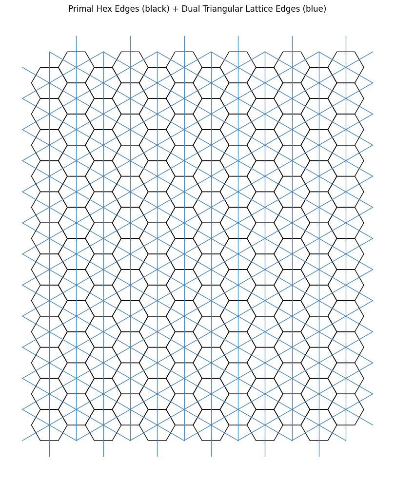
We start off where we left off in the Auxiliary Insights section of the last blog post.
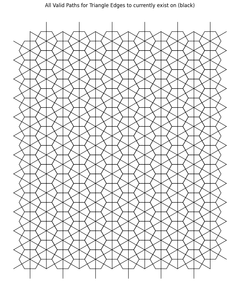
Recall that a rotation by \(60^\circ\) returns us to the original dual line due to the underlying sixfold symmetry. For the \(2\)-close interaction, we introduced a new dual by halving this angle to $30^\circ$. Naturally, to explore the \(3\)-close case, one might attempt the naive approach of halving again to $15^\circ$. However, as seen below, this approah does not yield the desired result, indicating that the simple halving approach cannot be extended straightforwardly.
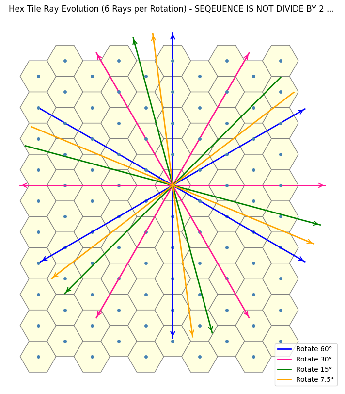
By manually guessing and checking the rotation values, we end up with a somewhat unexpected sequence, something that, for me at least, is nothing immediately obvious.
This hints at the need to uncover a more subtle structure that lets us analytically determine the values we seek.
Some prerequisite background is provided in the next section, but if you’re already familiar, feel free to skip ahead to the solution process that builds on these ideas.
Some useful underlying mathematics prerequisites that could help
Modular Arithmetic
A Quick Introduction to Modular Arithmetic
Modular arithmetic is a system of arithmetic for integers where numbers “wrap around” after reaching a certain value called the modulus. Rather than focusing on the full quotient of a division, modular arithmetic concerns itself with the remainder. It is a foundational concept in number theory and has wide applications in cryptography, computer science, and abstract algebra.
Motivation
Suppose you are working with a standard 12-hour clock. If the current time is 9 and 5 hours pass, the clock shows 2, not 14. This is because clocks operate “modulo 12”, meaning we consider two numbers equivalent if they differ by a multiple of 12. So:
$$
9 + 5 = 14 \equiv 2 \pmod{12}
$$
This is a basic example of modular arithmetic: rather than computing the full sum, we reduce it to its residue modulo 12.
Definition
Let \(n \) be a fixed positive integer, called the modulus. For any integers \(a \) and \(b \), we say:
$$
a \equiv b \pmod{n}
$$
(read as “a is congruent to b modulo n”) if and only if \(n \) divides \(a – b \); that is, there exists an integer \(k \) such that:
$$
a – b = kn
$$
This defines an equivalence relation on the set of integers \(\mathbb{Z} \), which partitions \(\mathbb{Z} \) into \(n \) distinct congruence classes modulo \(n \). Each class contains all integers with the same remainder upon division by \(n \).
For example, with \(n = 5 \), the integers are grouped into the following classes:
$$
[0] = { \dots, -10, -5, 0, 5, 10, \dots }
$$
$$
[1] = { \dots, -9, -4, 1, 6, 11, \dots }
$$
$$
[2] = { \dots, -8, -3, 2, 7, 12, \dots }
$$
$$
[3] = { \dots, -7, -2, 3, 8, 13, \dots }
$$
$$
[4] = { \dots, -6, -1, 4, 9, 14, \dots }
$$
Each integer belongs to exactly one of these classes. For computational purposes, we usually represent each class by its smallest non-negative element, i.e., by the residue \(r \in {0, 1, \dots, n-1} \).
Arithmetic in \(\mathbb{Z}/n\mathbb{Z} \)
The set of congruence classes modulo \(n \), denoted \(\mathbb{Z}/n\mathbb{Z} \), forms a ring under addition and multiplication defined by:
- \([a] + [b] := [a + b] \)
- \([a] \cdot [b] := [ab] \)
These operations are well-defined: if \(a \equiv a’ \pmod{n} \) and \(b \equiv b’ \pmod{n} \), then \(a + b \equiv a’ + b’ \pmod{n} \) and \(ab \equiv a’b’ \pmod{n} \).
If \(n \) is prime, \(\mathbb{Z}/n\mathbb{Z} \) is a finite field, meaning every nonzero element has a multiplicative inverse.
Formal Summary
Modular arithmetic generalizes the idea of remainders after division. Formally, for a fixed modulus \(n \in \mathbb{Z}_{>0} \), we say:
$$
a \equiv b \pmod{n} \iff n \mid (a – b)
$$
This defines a congruence relation on \(\mathbb{Z} \), leading to a system where calculations “wrap around” modulo \(n \). It is a central structure in elementary number theory, forming the foundation for deeper topics such as finite fields, Diophantine equations, and cryptographic algorithms.
Law Of Sines
Derivation of the Law of Sines
The Law of Sines is a fundamental result in trigonometry that relates the sides of a triangle to the sines of their opposite angles. This elegant identity allows us to find unknown angles or sides in oblique triangles using simple trigonometric ratios.
Setup and Construction
Consider an arbitrary triangle \(\triangle ABC \) with:
- \(a = BC \)
- \(b = AC \)
- \(c = AB \)
To derive the Law of Sines, we draw an altitude from vertex \(A \) perpendicular to side \(BC \), and denote this height as \(h \).
Now consider the two right triangles formed by this altitude:
- In \(\triangle ABC \), using angle \(B \): $$
\sin B = \frac{h}{a} \quad \Rightarrow \quad h = a \sin B
$$ - Using angle \(C \): $$
\sin C = \frac{h}{b} \quad \Rightarrow \quad h = b \sin C
$$
Since both expressions equal \(h \), we equate them:
$$
a \sin B = b \sin C
$$
Rewriting this gives:
$$
\frac{a}{\sin C} = \frac{b}{\sin B}
$$
We can repeat this construction by drawing altitudes from the other vertices to derive similar relationships:
$$
\frac{b}{\sin A} = \frac{c}{\sin B}, \quad \frac{c}{\sin A} = \frac{a}{\sin C}
$$
Combining all, we obtain the complete Law of Sines:
$$
\frac{a}{\sin A} = \frac{b}{\sin B} = \frac{c}{\sin C}
$$
Geometric Interpretation
The Law of Sines implies that in any triangle, the ratio of a side to the sine of its opposite angle is constant. In fact, this constant equals \(2R \), where \(R \) is the radius of the circumcircle of the triangle:
$$
\frac{a}{\sin A} = \frac{b}{\sin B} = \frac{c}{\sin C} = 2R
$$
This shows a deep geometric connection between triangles, circles, reflecting the underlying symmetry of some parts of Euclidean geometry.
Law Of Cosines (generalisation of Pythagorean theorem)
Derivation of the Cosine Angle Formula
The cosine angle formula, also known as the Law of Cosines, relates the lengths of the sides of a triangle to the cosine of one of its angles.
Motivation
Consider a triangle with sides of lengths \(a \), \(b \), and \(c \), and let \(\theta \) be the angle opposite side \(c \). When \(\theta \) is a right angle, the Pythagorean theorem applies:
$$
c^2 = a^2 + b^2
$$
For any angle \(\theta \), the Law of Cosines generalizes this relationship:
$$
c^2 = a^2 + b^2 – 2ab \cos \theta
$$
This formula allows us to find a missing side or angle in any triangle, not just right triangles.
Setup and Coordinate Placement
To derive the formula, place the triangle in the coordinate plane:
- Place vertex \(A \) at the origin \((0, 0) \).
- Place vertex \(B \) on the positive x-axis at \((b, 0) \).
- Place vertex \(C \) at \((x, y) \), such that the angle at \(A \) is \(\theta \).
By definition, the length \(a \) is the distance from \(B \) to \(C \), and \(c \) is the length from \(A \) to \(C \).
Since \(\theta \) is the angle at \(A \), the coordinates of \(C \) can be expressed using polar coordinates relative to \(A \):
$$
C = (a \cos \theta, a \sin \theta)
$$
Distance Calculation
The length \(c \) is the distance between points \(A(0,0) \) and \(C(a \cos \theta, a \sin \theta) \):
$$
c = \sqrt{(a \cos \theta – 0)^2 + (a \sin \theta – 0)^2} = a
$$
Actually, to keep consistent with the notation, let’s redefine:
- \(AB = c \)
- \(AC = b \)
- \(BC = a \)
So placing:
- \(A = (0, 0) \)
- \(B = (c, 0) \)
- \(C = (x, y) \)
with angle \(\theta = \angle A \) at point \(A \).
Point \(C \) has coordinates:
$$
C = (b \cos \theta, b \sin \theta)
$$
The length \(a = BC = \) distance between \(B(c, 0) \) and \(C(b \cos \theta, b \sin \theta) \):
$$
a^2 = (b \cos \theta – c)^2 + (b \sin \theta – 0)^2
$$
Expanding:
$$
a^2 = (b \cos \theta – c)^2 + (b \sin \theta)^2
= (b \cos \theta)^2 – 2bc \cos \theta + c^2 + b^2 \sin^2 \theta
$$
Simplify using the fundamental trigonometric identity \(\cos^2 \theta + \sin^2 \theta = 1 \):
$$
a^2 = b^2 \cos^2 \theta – 2bc \cos \theta + c^2 + b^2 \sin^2 \theta = b^2(\cos^2 \theta + \sin^2 \theta) – 2bc \cos \theta + c^2
$$
$$
a^2 = b^2 – 2bc \cos \theta + c^2
$$
This is the Law of Cosines, it states that for any triangle with sides \(a, b, c \) and angle \(\theta \) opposite side \(a \):
$$
a^2 = b^2 + c^2 – 2bc \cos \theta
$$
This formula generalizes the Pythagorean theorem and allows computation of unknown sides or angles in any triangle, making it fundamental in trigonometry and geometry.
Height of a Regular Hexagon of Side Length, \(a\)
Find the height of a regular hexagon with side length \(a\)
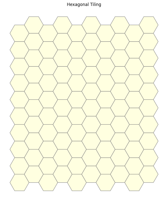
Understand the structure of a regular hexagon
- A regular hexagon can be divided into 6 equilateral triangles.
- Each triangle has side length \(a\).
- The height of the hexagon is the distance between two parallel sides, i.e., it’s twice the height of one equilateral triangle formed inside.
So:
$$
\text{height of hexagon} = 2 \times \text{height of equilateral triangle with side } a
$$
Use formula for height of an equilateral triangle
The height \(h\) of an equilateral triangle with side length \(a\) is:
$$
h = a \cdot \sin(60^\circ)
$$
We use this since the height splits the triangle into two right triangles with angles \(30^\circ, 60^\circ, 90^\circ\).
Substitute:
$$
\sin(60^\circ) = \frac{\sqrt{3}}{2}
$$
So:
$$
h = a \cdot \frac{\sqrt{3}}{2}
$$
Multiply by 2 to get full hexagon height
$$
\text{Height of hexagon} = 2 \cdot \left( a \cdot \frac{\sqrt{3}}{2} \right)
$$
Yielding Result:
$$
\text{Height of a regular hexagon with side length } a = a \sqrt{3}
$$
Limits at infinity
Limits at Infinity: A Conceptual Overview
In mathematical analysis, the notion of a limit at infinity provides a rigorous framework for understanding the behavior of functions as their input grows arbitrarily large in magnitude. Specifically, we are interested in the asymptotic behavior of a function \(f(x) \) as \(x \to \infty \) (or \(x \to -\infty \)), that is, how \(f(x) \) behaves for sufficiently large values of \(x \).
Formally, we say that
$$
\lim_{x \to \infty} f(x) = L
$$
if for every \(\varepsilon > 0 \), there exists a real number \(N \) such that
$$
x > N \Rightarrow |f(x) – L| < \varepsilon.
$$
This definition captures the idea that the values of \(f(x) \) can be made arbitrarily close to \(L \) by taking \(x \) sufficiently large.
Limits at infinity play a crucial role in the study of convergence, asymptotics, and the global behavior of functions.
Continuing to derive the solution
Simplifying the focus
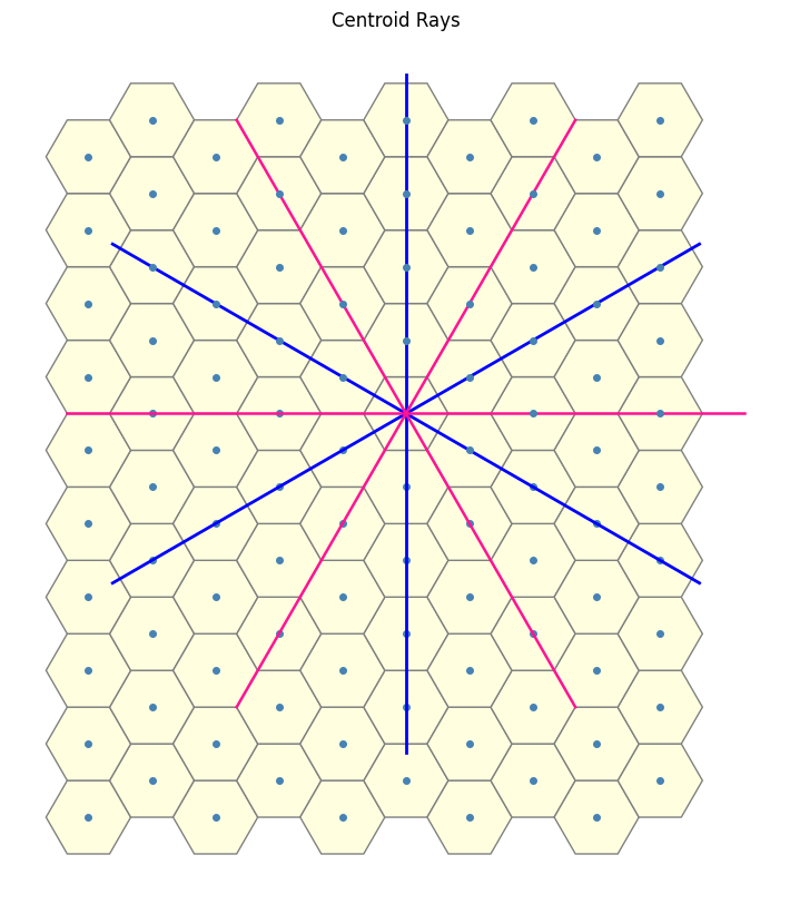
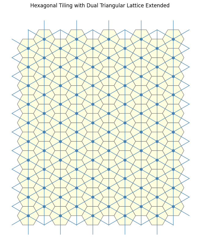
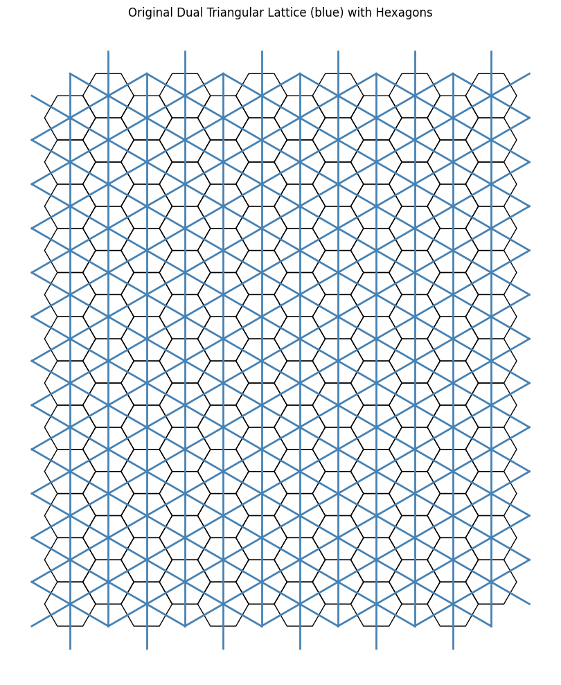
We begin by exploiting the inherent sixfold rotational symmetry, we reduce the problem “modulo 6”-style, effectively restricting our attention to a single fundamental sector (i.e one \(60\) degree sector). By doing so we simplify the analysis to just one representative section within this equivalence class.
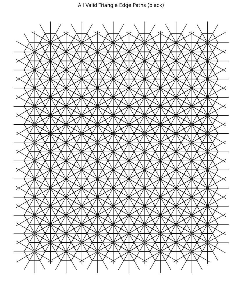
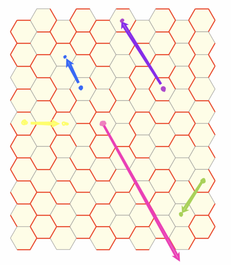
If we restrict our view to along the direction of the blue arrow, we observe that the rotation lines align to form a straight “line” sequence. This linear arrangement reveals an underlying order that we can potentially use.
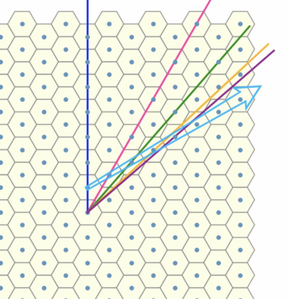
To proceed, we now seek an invariant, a quantity or structure that remains stable under the transformations, under consideration. The natural approach here is to introduce an auxiliary red arrow, aligned with the reference direction. By connecting this to each rotation line, we form triangles with a common “base”.
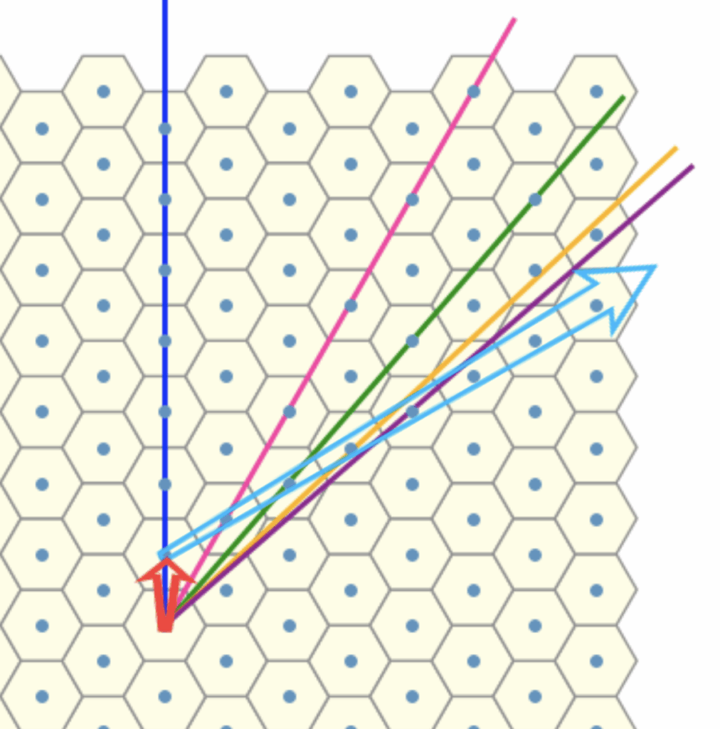
Let us now regard each line as encoding an angular offset, specifically, a rotation relative to a fixed reference direction given by the dark blue line (dual). , We can think of the red arrow as some sort of basis vector corresponding to the blue line . Our aim is to compute the rotational offset of each line with respect to this reference frame, treating the red arrow as a canonical representative of the direction encoded by the dark blue line.
Finding the general formula for the offset angle between the red arrow (a representation of the original dual) AND the \(n\)-case triangle

Given:
- Triangle with two sides:
- Side 1: \(a \sqrt{3}\)
- Side 2: \(a n \sqrt{3}\)
- Included angle between them: \(120^\circ\)
- Goal: Find the angle \(A\), opposite to the side \(a n \sqrt{3}\)
Step 1: Use Law of Cosines to find the third side
$$
c^2 = \alpha^2 + \beta^2 – 2 \alpha \beta \cos(C)
$$
Assign:
- \( \alpha = a \sqrt{3}\)
- \(\beta = a n \sqrt{3}\)
- \(C = 120^\circ\)
$$
c^2 = (a \sqrt{3})^2 + (a n \sqrt{3})^2 – 2 (a \sqrt{3})(a n \sqrt{3}) \cos(120^\circ)
$$
Evaluate:
- \((a \sqrt{3})^2 = 3 a^2\)
- \((a n \sqrt{3})^2 = 3 a^2 n^2\)
- \(2ab = 6 a^2 n\)
- \(\cos(120^\circ) = -\frac{1}{2}\)
$$
c^2 = 3 a^2 + 3 a^2 n^2 + 3 a^2 n
$$
$$
c^2 = 3 a^2 (n^2 + n + 1)
$$
$$
c = a \sqrt{3 (n^2 + n + 1)}
$$
Step 2: Use Law of Sines to find the angle opposite to \(a n \sqrt{3}\)
$$
\frac{\sin A}{a n \sqrt{3}} = \frac{\sin(120^\circ)}{c}
$$
Substitute:
- \(\sin(120^\circ) = \frac{\sqrt{3}}{2}\)
- \(c = a \sqrt{3 (n^2 + n + 1)}\)
$$
\sin A = \frac{a n \sqrt{3}}{a \sqrt{3 (n^2 + n + 1)}} \times \frac{\sqrt{3}}{2}
$$
Cancel \(a\):
$$
\sin A = \frac{n \sqrt{3}}{\sqrt{3 (n^2 + n + 1)}} \times \frac{\sqrt{3}}{2}
$$
$$
\sin A = \frac{3 n}{2 \sqrt{3 (n^2 + n + 1)}}
$$
Final Result for the ? angle:
$$
A = \sin^{-1} \left( \frac{3 n}{2 \sqrt{3 (n^2 + n + 1)}} \right)
$$
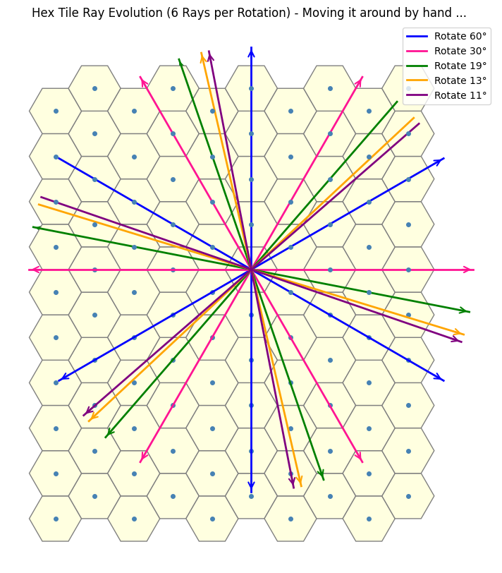
Adjusting the Sequence for clearer understanding of the Asymptotics
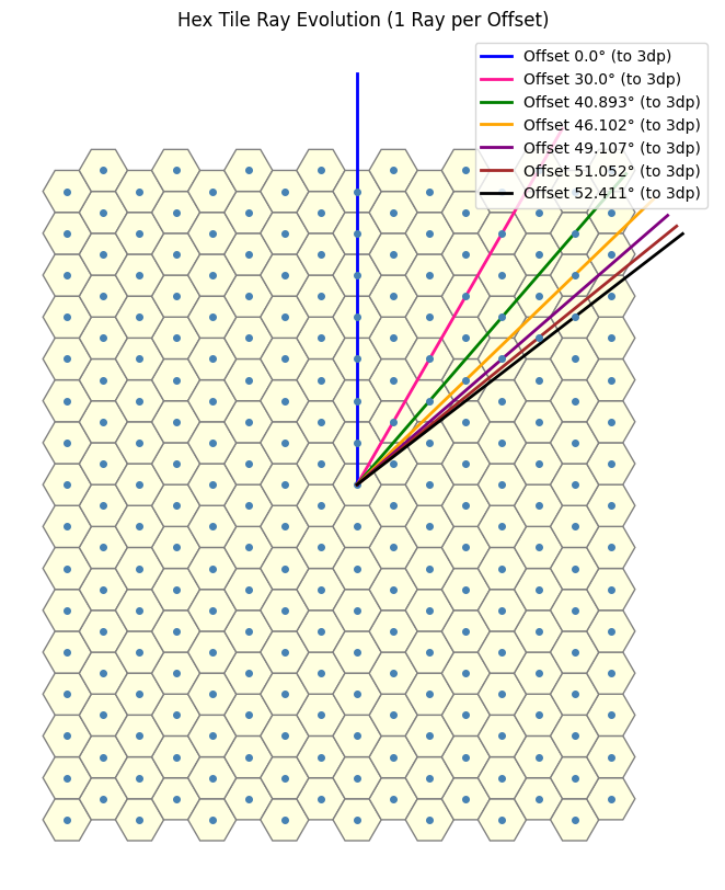
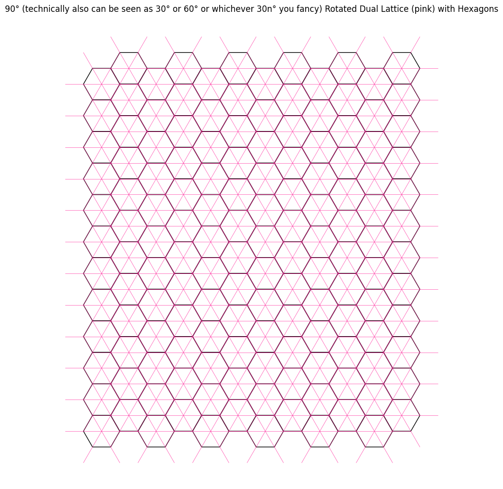
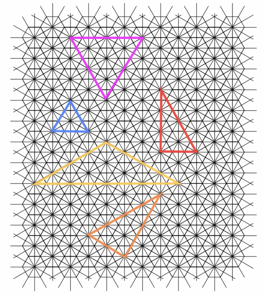
We can now utilize the function defined above to generate the desired terms in the sequence. This brings us close to our objective. Upon closer inspection, we observe that the sequence aligns particularly well when interpreted as an angular offset. Specifically, as illustrated in the image below, we begin with the blue line corresponding to the case \(n = 0\), and for each subsequent value of \(n\), we proceed in a clockwise direction. (These lines correspond to the dotted rays shown in the previous image.)
Drawing a link between the symmetry and this
Originally, by leveraging the underlying symmetry of the problem, we simplified the analysis by focusing in a single direction, meaning in other words, we can intuitively infer that the sequence “resets” every 60 degrees.
Now instead, we can analyze the limiting behavior of the relevant angle in the \(n\)-th triangle considered earlier. As \(n\) grows large, the angle opposite the red line (the \(a \sqrt{3}\) side), which we denote by \(\omega\), decreases towards zero. Formally, this can be expressed as
$$
\lim_{n \to \infty} \omega = 0.
$$
Using the triangle angle sum formula, the angle of interest (the ?, but lets call it \(\phi\)), satisfies
$$
\phi = 180^\circ – 120^\circ – \omega.
$$
Therefore,
$$
\lim_{n \to \infty} \phi = 60^\circ,
$$
showing that the sequence converges to \(60^\circ\).
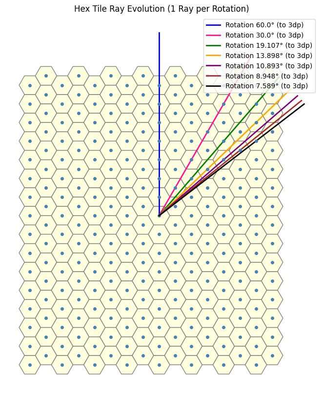
Final Adjustment of the formula to reflect the rotation of the original dual and the intuition above
Thus, from both a mathematical (okay maybe more so an aesthetic) standpoint, it is preferable to redefine the sequence so that it converges to zero. This aligns with the conceptual goal of determining ‘how much to rotate’ the original dual structure to obtain the \(n\)-th dual. In its current form, the sequence converges to a fixed offset (specifically, \(60^\circ\)), which, at first glance, is not immediately apparent from the formula.
To clarify what is meant by ‘converging to zero’: when we rotate the original dual by any multiple of \(60^\circ\) (i.e., an element of \(60\mathbb{Z}\)), we return to the original dual; similarly, a rotation by \(30\mathbb{Z}\) yields the 2-close interaction. In this context, we seek a rotation angle \(\theta\) such that \(\theta \cdot \mathbb{Z}\) captures the \(n\)-close interaction, and thus, it is natural to define \(\theta\) as a function of \(n\) that tends to zero as \(n \to \infty\). This reframing reveals the underlying structure more clearly and places the emphasis on the relative rotation required to reach the \(n\)-th configuration from the base case.
This sequence tending to zero carries a natural interpretation: it suggests diminishing deviation or adjustment over time. This aligns well with the intuition that as \(n\) increases, the system or pattern is “settling down” or tending to the reset point. In contrast, convergence to a nonzero constant may obscure this interpretation (unless you know a-priory about the symmetries of this system) , since the presence of a persistent offset implies a kind of residual asymmetry or imbalance. By ensuring that the sequence vanishes asymptotically, we emphasize convergence toward a limiting behavior centered at zero.
This was the justification to introducing a subtraction of 60 in front of the A earlier to consider the sequence in the original notion of rotation of the dual instead. Yielding us
$$
\theta = 60 \ – \ A
$$
$$
\theta = 60 \ – \ \sin^{-1} \left( \frac{3 n}{2 \sqrt{3 (n^2 + n + 1)}} \right).
$$
After this adjustment, hopefully it becomes apparent, even from a quick inspection of the formula, that the constant \(60\) plays a fundamental role in limiting structure of the problem.
Thus we have
The Problem is not finished
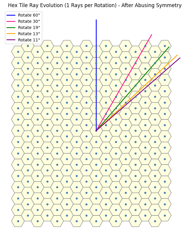
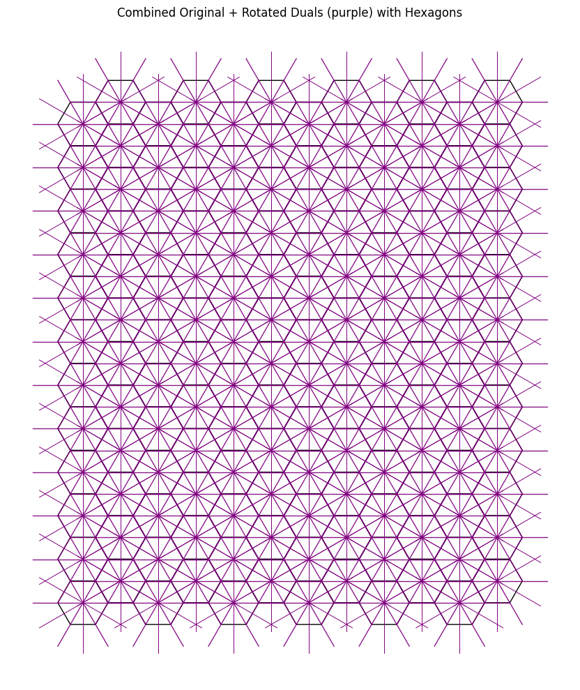
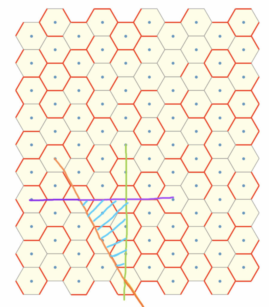
Now, reintroducing the 6-fold symmetry and examining the superposition of plots corresponding to the 1-close through \(n\)-close interactions (for increasingly large values of \(n\)), we observe:
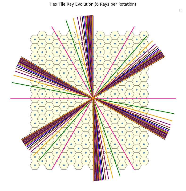
But wait … this does not cover the full grid. It’s clearly missing parts! You scammed me! Well yes but not quite as I did mention at the start
“…closed-form starting step”
Srivathsan Amruth,
You really didn’t think I was going to give you the full answer right…
I intentionally stopped here, as I want you to explore the problem further and realize that there are, in fact, additional symmetries you can exploit to fully cover the hexagonal grid. I’ll leave you with a the following hint to start:
Consider the 1-ray case and its associated \(60^\circ\) cone.
Now look at the 3-close case (green) and the 2-close case (purple). Ask yourself: can I flip something to fill in the missing part of the 3-close structure?
Then, move on to the 4-close case. Since (spoiler) there will be two distinct 3-close components involved, can I once again use flipping to complete the picture? And if so, how many times, and where, should these flips occur?
It’s getting quite recursive from here… but I’ll let you figure out the rest.
Also, I’ll leave you with one final thought, i.e is there a way to avoid this recursive construction altogether or simplify the approach, and instead generate the full structure more efficiently using some iterative or closed-form approach?
Wishing you a hex-tra special day ahead with every piece falling neatly into place.
Srivathsan Amruth,
i.e The personguidingoffering youthroughthis symmetry-induced spiral.


