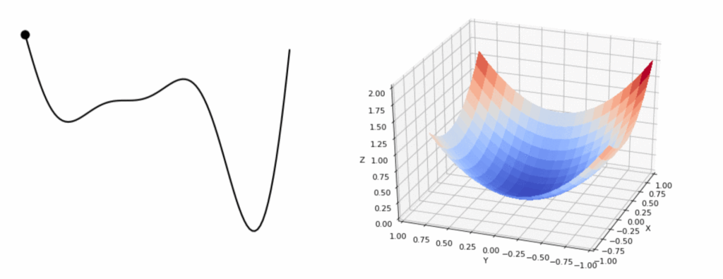
Picture your triangle mesh as that poor, crumpled T-shirt you just pulled out of the dryer. It’s full of sharp folds, uneven patches, and you wouldn’t be caught dead wearing it in public—or running a physics simulation! In geometry processing, these “wrinkles” manifest as skinny triangles, janky angles, and noisy curvature that spoil rendering, break solvers, or just look… ugly. Sometimes, we might want to fix these problems using something geometry nerds call surface fairing.
Figure 1. (Left) Clean mesh, (Right) Mesh damaged by adding Gaussian noise to each vertex (Middle) Result after applying surface fairing to the damaged mesh.
In essence, surface fairing is an algorithm one uses to smoothen their mesh. Surface fairing can be solved using energy minimization. We define an “energy” that measures how wrinkly our mesh is, then use optimization algorithms to slightly nudge each vertex so that the total energy drops.
Spring Energy Think of each mesh edge (i,j) as a spring with rest length 0. If a spring is too long, it costs energy. Formally: Emem = ½ Σ(i,j)∈E wij‖xi − xj‖² with weights wij uniform or derived from entries of the discrete Laplacian matrix (using cotangents of opposite angles). We’ll call this term the Membrane Term
Bending Energy Sometimes, we might want to additionally smooth the mesh even if it looks less wrinkly. In this case, we penalize the curvature of the mesh, i.e., the rate at which normals change at the vertices: Ebend = ½ Σi Ai‖Δxi‖² where Δxi is the discrete Laplacian at vertex i and Ai is its “vertex area”. For the uninitiated, the idea of a vertex having an area might seem a little weird. But it represents how much area a vertex controls and is often calculated as one-third of the summed areas of triangles incident to vertex i. We’ll call this energy term the Laplacian Term.
Angle Energy As Nicholas has warned the fellows, sometimes, having long skinny triangles can cause numerical instability. So we might like our triangles to be more equilateral. We can additionally punish deviations from 60° for each triangle, by adding another energy term: Eangle = Σk=1..3(θk−60°)². We’ll call this the Angle Term.
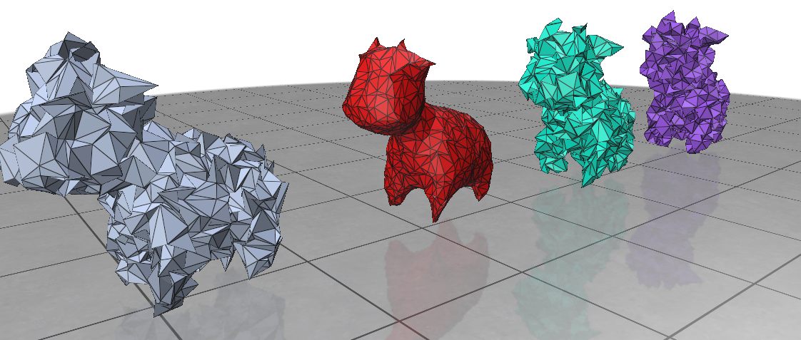
Figure 2. (Left) Damaged mesh. (In order) Surface fairing using only 1) Spring Energy 2) Bending Energy 3) Angle Energy. Notice how the last two energy minimizations fail to smooth the mesh properly alone.
Note that in most cases using angle energy and bending energy terms are optional, but using the spring energy term is important! (however, you may encounter a few special cases where you can make do without the spring energy?? i’m not too sure, don’t take my word for it). Once we have computed these energies, we weight them appropriately with scaling factors and sum them up. The next step is to minimize them. I love Machine Learning and hate numerical solvers; and so, it brings me immense joy to inform you that since the problem is non-convex, we can should use gradient descent! At each vertex, compute the gradient ∇xE and take a tiny step towards the minima: \(x_{i} \leftarrow x_i – \lambda \cdot (\nabla_{x} E)_{i}\)
Now, have a look at our final surface fairing algorithm in its fullest glory. Isn’t it beautiful? Maybe you and I are nerds after all 🙂
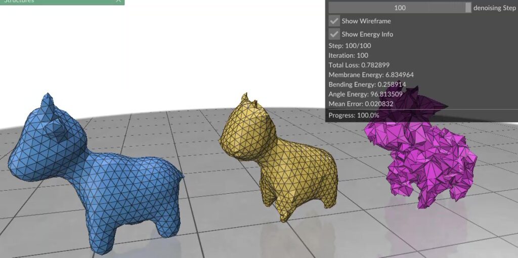
Figure 1. (Left) Clean mesh, (Right) Damaged mesh (Middle) Resulting mesh after each step of gradient descent on the three energy terms combined. Note how the triangles in this case are more equilateral than the red mesh in Figure 2, because we’ve combined all energy terms.
So, the next time your mesh looks like you’ve tossed a paper airplane into a blender, remember: with a bit of math and a few iterations, you can make it runway-ready; and your mesh-processing algorithm might just thank you for sparing its life. You can find the code for the blog at github.com/ShreeSinghi/sgi_mesh_fairing_blog.
Happy geometry processing!
References
Desbrun, M., Meyer, M., Schröder, P., & Barr, A. H. (1999). Implicit fairing of irregular meshes using diffusion and curvature flow.
Pinkall, U., & Polthier, K. (1993). Computing discrete minimal surfaces and their conjugates.
Now that you’ve gotten the grasp of meshes, and created your very first 3D object on Polyscope, what can we do next? On Day 4 of the SGI Tutorial Week, we had speakers Richard Liu and Dale Decatur from the Threedle Lab at UChicago explaining about Texture Optimization.
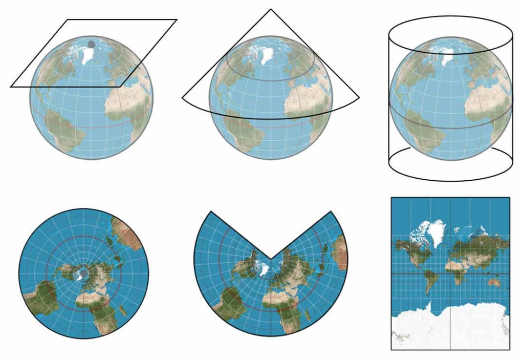
In animated movies and video games, we are used to observing them with realistic textures. Intuitively, we might imagine that we have this texture as a map applied as a flat “sticker” over it. However, we know from some well-known examples in cartography that it is difficult to create a 2D map of a 3D shape like the Earth without introducing distortions or cuts.
Besides, ideally, we would want to be able to transition from the 2D to the 3D map interchangeably. Framing this 2D map as a function on \(\mathbb{R^2}\), we would like it to be bijective.
The process of creating a bijective map from a mesh S in \(\mathbb{R^3}\) to a given domain \(\Omega\), or \(F: \Omega \leftrightarrow S\), is known as mesh parametrization.
Consider a mesh defined by the object as \(M = {V, E, F}\), with Vertices, Edges and Faces respectively, where:
\begin{equation*}
V \subset R^3
\end{equation*}
\begin{align*}
E = \{(i, j) \quad &| \text{\quad vertex i is connected to vertex j}\} \\
F = \{(i, j, k) \quad &| \quad \text{vertex i, j , k share a face}\}
\end{align*}
For a mesh M, we define the parametrization as a function mapping vertices \(V\) to some domain \(\Omega\)
\begin{equation*}
U: V \subset \mathbb{R}^3 \rightarrow \Omega \subset \mathbb{R}^2
\end{equation*}
For every vertex \(v_i\) we assign a 2D coordinate \(U(v_i) = (u_i, v_i)\) (this is why the method is called UV unwrapping).
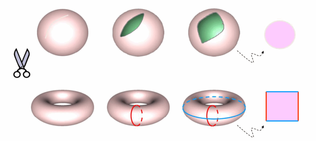
This parametrization has a constraint, however. Only disk topology surfaces (those with a 1 boundary loop) surfaces admit a homeomorphism (a continuous and bijective map) to the bounded 2D plane.
Source: Richard Liu
As a workaround, we can always introduce a cut.
Source: Richard Liu
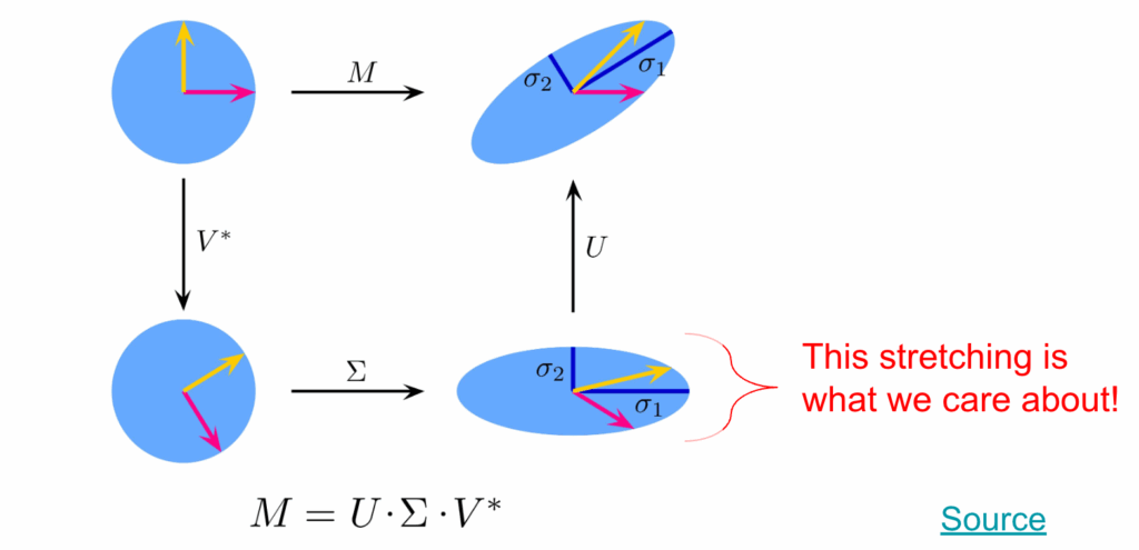
However, these seams create discontinuities, and in turn, distortions we want to minimize. We can distinguish different kinds of distortions using the Jacobian, the matrix of all first-order partial derivatives of a vector-valued function. Specifically, we look at the singular values of the Jacobian (which in the UV function is defined as a 2×3 matrix per triangle).
\begin{align*}
J_f = U\Sigma V^T = U \begin{pmatrix}
\sigma_1 & 0 \\
0 & \sigma_2 \\
0 & 0
\end{pmatrix} V^T \\
f \text{ is equiareal or area preserving} \Leftrightarrow \sigma_1 \sigma_2 &= 1 \\
f \text{ is equiareal or area preserving} \Leftrightarrow \sigma_1 &= \sigma_2 \\
f \text{ is equiareal or area preserving} \Leftrightarrow \sigma_1 &= \sigma_2 = 1
\end{align*}
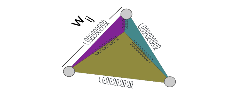
The classical approach for optimizing a mesh parametrization is viewing the mesh surface as the graph of a mass-spring system (least squares optimization problem). The mesh vertices are the nodes (with equal mass) with each edge acting as a spring with some stiffness constant.
Source: Richard Liu
Two key design choices in setting up this problem are:
Where to put the boundary?
How to set the spring weights (stiffness)?
To compute the parametrization, we minimize the sum of spring potential energies.
Where \(N_i\) indexes all neighbors of vertex \(i\). We can now fix the boundary vertices and solve each equation for the remaining \(u_i\).
A solution by Tutte (1963) and Floater (1997) was computed such that if the boundary is convex and the weights are positive, the solution is guaranteed to be injective. While an injective map has its limitations in terms of transferring the texture back into the 3D shape, it allows us to easily visualize the 2D map of this shape.
Here, we would need to fix or map a boundary to a circle, where all weights are 1.
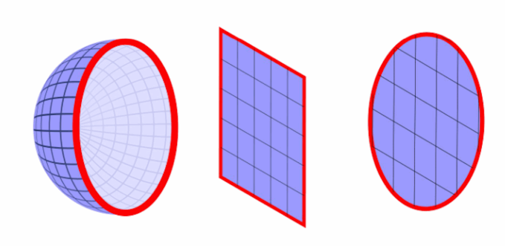
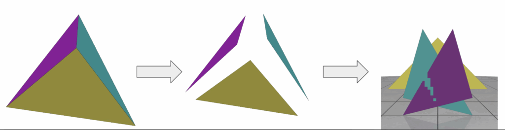
An alternative to the classical approach is trivial parametrization, where we split the mesh up into its individual triangles in a triangle soup and then flatten each triangle (isometric distortion). We would then translate and scale all triangles to be packed into the unit square.
Source: Richard Liu
Translation and uniform scaling does not affect the angles, such that we have no angle distortion. So this tells us that this parametrization approach is conformal.
Still, when packing triangles into the texture image, we might need to rescale them so they fit, meaning the areas are not guaranteed to be the same. We can verify this based on the SDF values:
This won’t be too relevant in the end though because all triangles get scaled by the same factor, so that the area of each triangle is preserved up to some global scaler. As a result, we would still get an even sampling of the surface, which is what we would care about, at least intuitively, for texture mapping.
However, applying a classical algorithm to trivial parametrization is typically a bad solution because it introduces maximal cuts (discontinuities). How can we overcome this issue?
Parametrization with Neural Networks
Assume we have some parametrized function and some target value. With an adaptive learning algorithm, we determine the direction in which to change our parameters so that the function moves closer to our target.
We compute some loss or measure of closeness between our current function evaluation and our target value.We then compute the gradient of this loss with respect to our parameters. Take a small step in that direction. We would repeat this process until we ideally achieved the global minimum.
Target = existing images of the object with the desired colors
Loss = pixel differences between our rendered images and target images.
What happens if we do this? We do achieve a texture map, but each pixel is mostly optimized independently. As a result, the texture ends up more grainy.
Source: Dale Decatur
Improving Smoothness
What can we do to improve this? Well, we would want to make the function more smooth. For this, we can optimize a new function \(\phi(u, v) : \mathbb{R}^2 \rightarrow \mathbb{R}^2\) that maps the texels to RGB color values. By smoothness in \(\phi\), we mean that \(\phi\) is continuous.
To get the color at any point in the 2D texture map, we just need to query \(\phi\) at that UV coordinate!
Source: Dale Decatur
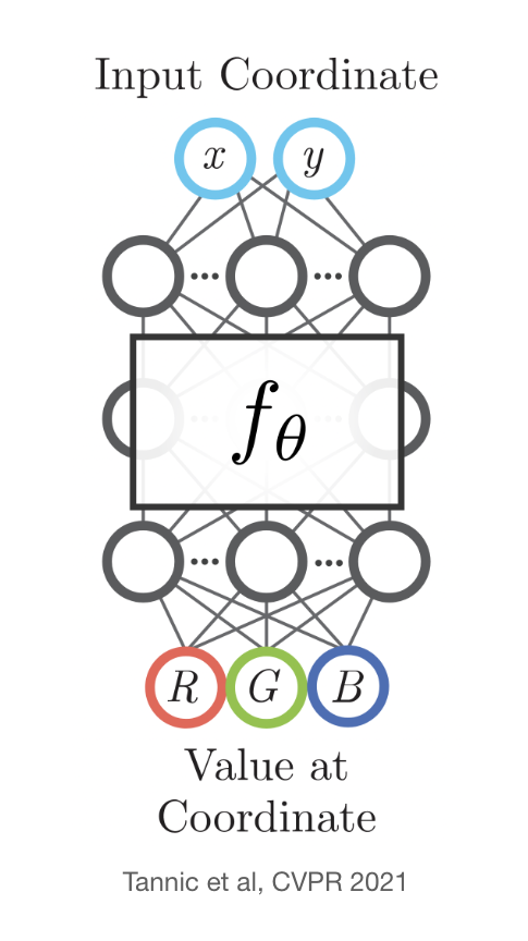
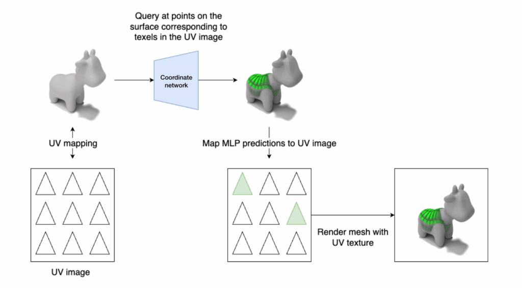
To encourage smoothness in \(\phi\), we can use a 3D coordinate network.
Tannic et al, CVPR 2021
Consider a mapping from a 3D surface to a 2D texture. We can learn a 3D coordinate \(\phi\): \(\mathbb{R}^3 \rightarrow \mathbb{R}^2\) that maps 3D surface points to RGB colors. \(\phi(x, y, z) = (R, G, B)\).
We can then use the inverse map to go from 2D texture coordinates to 3D surface points, then query those points with the coordinate network to get colors, then map those colors back to the 2D texture for easy rendering.
Source: Dale Decatur
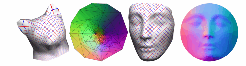
How to compute an inverse map?
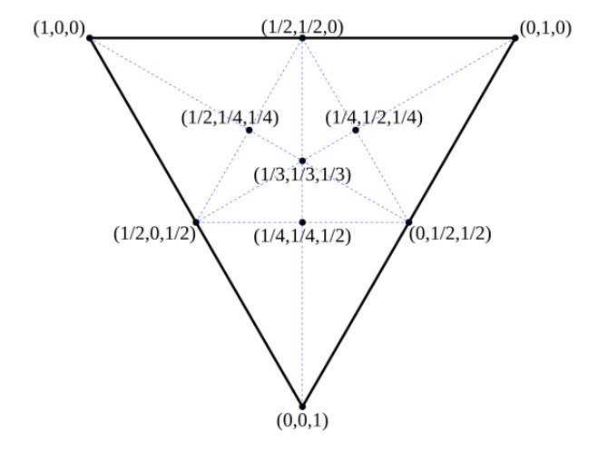
We aim to have a mapping from texels to surface poitns, but we already have a mapping from the vertices to the texel plane. The way we can map an arbitrary coordinate to the surface is through barycentric interpolation, a coordinate system relative to a given triangle. In this system, any points has 3 barycentric coordinates.
On July 11th, Nicholas Sharp, the creator of the amazing Polyscope library, gave the SGI Community an insightful talk on debugging and robustness in geometry processing—insights that would later save several fellows hours of head-scratching and mental gymnastics. The talk was broadly organized into five parts, each corresponding to a paradigm where bugs commonly arise:
Representing Numbers
Representing Meshes
Optimization
Simulation and PDEs
Geometric Machine Learning
Representing Numbers
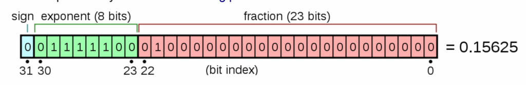
The algorithms developed for dealing with geometry are primarily built to work with clean and pretty real numbers. However, computers deal with floats, and sometimes they behave ugly. Floats are computers’ approximations of real numbers. Sometimes, it may require an infinite amount of storage to correctly represent a single number of arbitrary precision (unless you can get away with \(π=3.14\)). Each floating number can either be represented using 32 bits (single precision) or 64 bits (double precision).
Figure 1. An example of the float32 representation
In the floating realm, we have quirks like:
\((x+y)+z \neq x+(y+z)\)
\( a>0, b>0\) but \(a+b=a\)
It is important to note that floating-point arithmetic is not random; it is simply misaligned with real arithmetic. That is, the same operation will consistently yield the same result, even if it deviates from the mathematically expected one. Possible alternatives to floats are integers and binary fraction representations; however, they come with their own obvious limitations.
Who’s your best friend? The NaN! The NaN is a special “floating-point” computers spit out when they’re asked to perform invalid operations like
\(\frac{0}{0}\rightarrow \) NaN
\(\sqrt{-1} \rightarrow\) NaN (not \(i\) haha)
Every operation against a NaN results in… NaN. Hence, one small slip-up in the code can result in the entire algorithm being thrown off its course. Well then… why should I love NaNs? Because a screaming alarm is better than a silent error. If your algorithm is dealing with positive numbers and it computes \(\sqrt{-42}\) somewhere, you would probably want to know if you went wrong.
Well, what are some good practices to minimize numerical error in your code?
Don’t use equality for comparison, use thresholds like: \(\left| x – x^* \right| < \epsilon\) or \(\frac{\left| x – x^* \right|}{\left| x^* \right|} < \epsilon\)
Avoid transcendental functions wherever possible. A really cool example of this is to avoid \(\theta = \arccos \left( \frac{ \mathbf{u} \cdot \mathbf{v} }{ \left| \mathbf{u} \right| \left| \mathbf{v} \right| } \right)\) and use \(\cot \theta = \frac{ \cos \theta }{ \sin \theta } = \frac{ \mathbf{u} \cdot \mathbf{v} }{ \left| \mathbf{u} \times \mathbf{v} \right| }\) instead.
Clamp inputs to safe bounds, e.g. \(\sqrt{x} \rightarrow \sqrt{max(x, 0)}\). (Note that while this keeps your code running smoothly, it might convert NaNs into silent errors!)
Perturb inputs to singular functions to ensure numerical stability, e.g. \(\frac{1}{\left| x \right|} \to \frac{1}{\left| x \right| + \epsilon}\)
Some easy solutions include:
Using a rational arithmetic system, as mentioned before. Caveats include: 1) no transcendental operations 2) some numbers might require very large integers to represent them, leading to performance issues, in terms of memory and/or speed.
Use robust predicates for specific functional implementations, the design of which is aware of the common floating-point problems
Representing Surface Meshes
Sometimes, the issue lies not with the algorithm but with the mesh itself. However, we still need to ensure that our algorithm works seamlessly on all meshes. Common problems (and solutions) include:
Unreferenced vertices and repeated vertices: throw them out
A mixture of quad and triangular meshes: subdivide, retriangulate, or delete
Degenerate faces and spurious topology: either repair these corner cases or adjust the algorithm to handle these situations
Non-manifold and non-orientable meshes: split the mesh into multiple manifolds or orientable patches
Foldover faces, poorly tessellated meshes, and disconnected components: use remeshing algorithms like Instant Meshes or use Generalized Winding Numbers instead of meshes
Optimization
Several geometry processing algorithms involve optimization of an objective function. Generally speaking, linear and sparse linear solvers are well-behaved, whereas more advanced methods like gradient descent or non-linear solvers may fail. A few good practices include:
Performing sanity checks at each stage of your code, e.g. before applying an algorithm that expects SPD matrices, check if the matrix you’re passing is actually SPD
When working with gradient-descent-like solvers, check if the gradient magnitudes are too large; that may cause instability for convergence
Simulations and PDEs
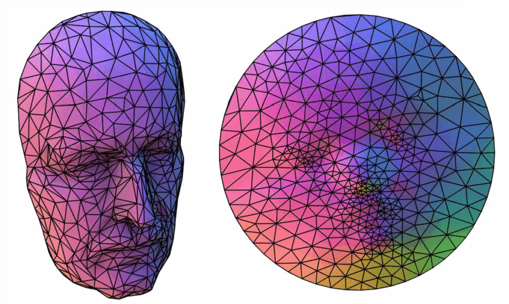
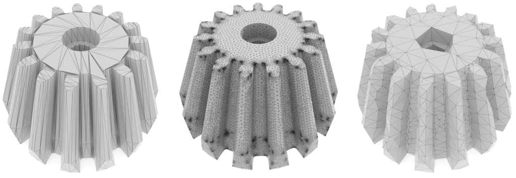
Generally, input meshes and algorithms are co-designed for engineering and scientific computing applications, so there aren’t too many problems with their simulations. However, visual computing algorithms need to be robust to arbitrary inputs, as they are typically just one component of a larger pipeline. Algorithms often fail when presented with “bad” meshes, even if it is perfect in terms of connectivity (like being a manifold, being oriented, etc.). Well then, what qualifies as a bad mesh? Meshes with skinny or obtuse triangles are particularly problematic. The solution is to remesh them using more equilateral triangles
Figure 2. (Left) An example of a “bad” mesh with skinny triangles. (Middle) A high-fidelity re-mesh that might be super-expensive to process. (Right) A low-fidelity re-mesh that trades fidelity for efficiency.
Geometric Machine Learning
Most geometric machine learning stands very directly atop geometry processing; hence, it’s important to get it right. The most common problems encountered in geometric machine learning are not so different from those encountered in standard machine learning. These problems include:
Array shape errors: You can use the Python aargh library to monitor and validate tensor shapes
NaNs and infs: Maybe your learning rate is too big? Maybe you’re passing bad inputs into singular functions? Use torch.autograd.set_detect_anomaly(mode, check_nan=True) to track these problematic numbers at inception.
“My trained model works on shape A, but not shape B.”: Is your normalization, orientation, and resolution consistent?
It is a good idea to overfit your ML model on a single shape and ensure that it works on simple objects like cubes and spheres before moving on to more complex examples.
And above all, the golden rule when your algorithm fails: Visualize everything.