Category: Uncategorized

🎭 A Tale of Two Transports: A Comic Drama in Three Acts 🎭

Dramatis Personae

• King Louis XVI — monarch of France; dislikes chaos and prefers order.
• Peasant — voice of everyday inefficiency.
• Gaspard Monge — French mathematician; formulates transport as a deterministic map with elegant clarity.
• Party Official — a bureaucrat, loves words like “plan.”
• Leonid Kantorovich — Soviet mathematician; introduces the convex relaxation that makes transport broadly solvable.
• Yann Brenier — mathematician; shows when the optimal plan is in fact a gradient map of a convex potential.

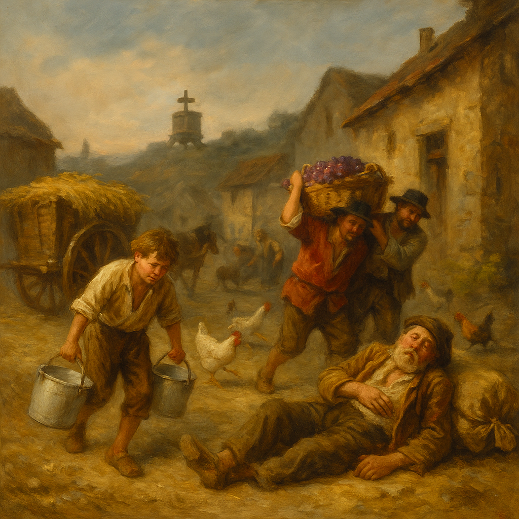
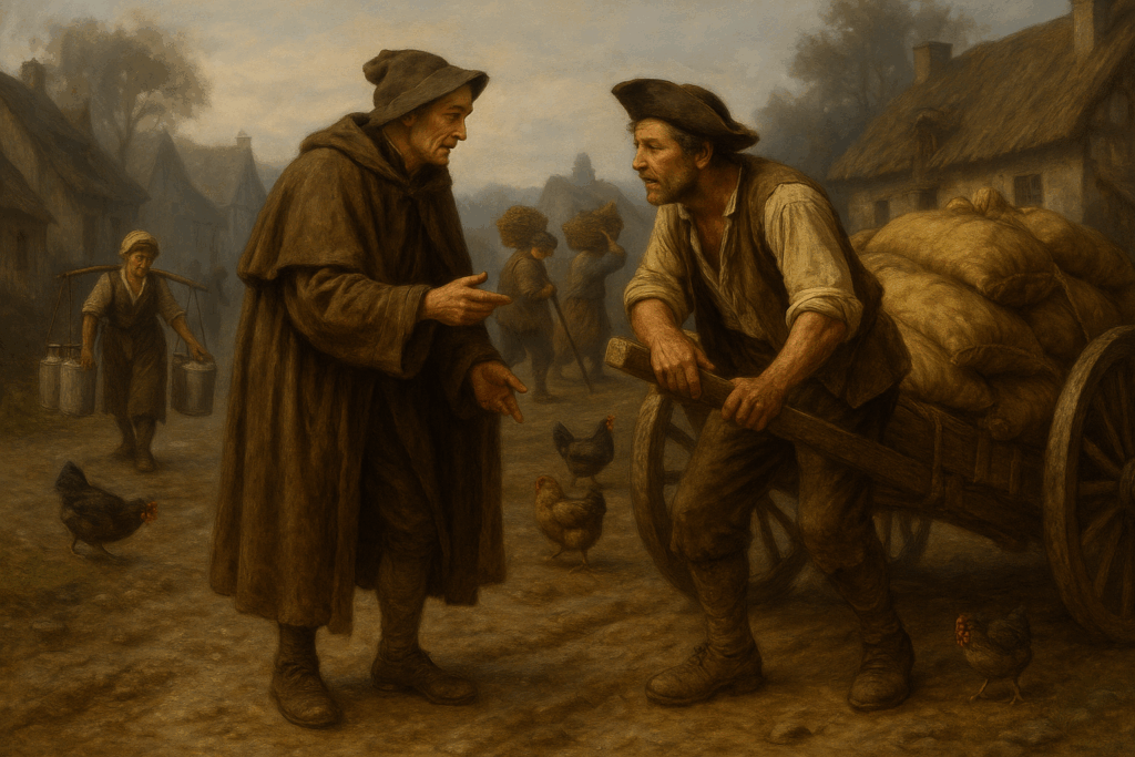
Act I — A Village in France, 1780

Scene: Grey dawn. Carts piled with wheat creak by; a boy staggers under chiming milk pails; two men shoulder grapes toward a wine press heroically far from grapes. Chickens run quality assurance on everyone’s ankles. A Peasant collapses onto a sack. Enter Louis XVI, in a plain cloak, incognito, attempting “peasant walk.”

👑 Louis XVI (softly, to himself): Ah, the countryside—so tranquil. (A wheelbarrow nearly flattened him.) … Enchanting.

“Pourquoi,” the Louis XVI asked a peasant who had stopped to breathe—and to reconsider his life choices—“is everyone running like headless hens? Why must you drag wheat halfway across France?”

👨‍🌾Peasant (gasping): New regulations—( he does not recognize him)—each farm must send all its wheat to the Rouen mill. Jean’s milk goes all beyond the river. Pierre’s grapes go all to that press on Mount Ridicule. Each farm is assigned to a factory regardless of whether it’s nearby or not. It is the system.

👑 Louis XVI (deadpan): System. Like umbrellas made of lace.

👨‍🌾 Peasant: They call it “Rational Logistics.” The rational part is the paperwork. The logistics we do on foot.

👑 Louis XVI : And why not send wheat to the nearest mill?

👨‍🌾Peasant: Nearest? (laughs, a little unwell) The Committee for Extended Journeys of Grain has determined “nearest” is bourgeois. We ship by destiny, not distance.

👨‍🌾Peasant (rising, grimly cheerful): Must be off. My route goes past Rouen, then back past here, then past my grave, then the mill.

👑 Louis XVI : Bon voyage. (beat) And bon sens… someday.

The Peasant trundles away, pursued by chickens. The King stares at the chaos like a man realizing his kingdom is a long proof with a missing lemma. He turns on his heel. Exit Louis XVI.

At the Royal Palace

Scene: A long table buried in maps. Brass compasses glint. Officials murmur in hexagons, puzzled. Enter Monge, ink on cuffs; Louis XVI presides.

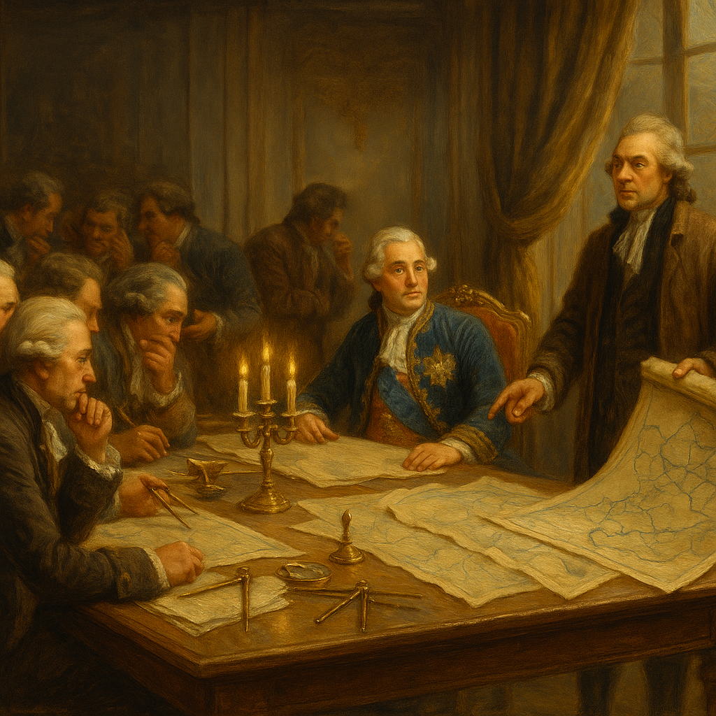
👑 Louis XVI (curt): The villages in France are ruled by chaos. Help us fix it.

Monge (with the unstoppable serenity of a man who believes the world can be improved by equations.): The problem is assigning yields (wheat, milk, grapes) from farms in France to the appropriate factories (flour mills, dairies, wine presses) at minimal total transport cost. That is optimal transport similar to the one with mines and factories that I was working on. Let me show you how to solve it with wheat and mills.

Monge (to Louis XVI ): Let us treat the country map as two mathematical worlds: \(X\) for farms and \(Y\) for mills. Plainly, \(Y\) and \(X\) are just set of points on your map (farm and mill locations), and any blob you can draw around those points is a region in which we might count wheat or capacity.

Precisely, take \(X\) and \(Y\) \( \in \mathbb{R}^2 \) (the plane of the map) and equip them with their restricted Borel \(\sigma\) -algebras:
\[
\mathcal{B}_X:=\{U\cap X:\ U\text{ open in }\mathbb{R}^2\},\qquad
\mathcal{B}_Y:=\{V\cap Y:\ V\text{ open in }\mathbb{R}^2\}.
\]
And there you have two measurable spaces: \((X,\mathcal{B}_X)\) and \((Y,\mathcal{B}_Y)\)

These \(\sigma\)-algebras specify which regions count as the measurable regions on which amounts can be tallied; the individual farm/mill points are measurable singletons and will serve as atoms.

Atomic data and finite Borel measures.
Given farms at points \(x_i\in X\) with supplies \(s_i\ge0\) and mills at points \(y_j\in Y\) with capacities
\(d_j\ge0\), define finite Borel measures (here \(\delta_x\) is the Dirac unit mass at \(x\)):
\[
\tilde\mu=\sum_i s_i \, \delta_{x_i}\\ \text{on}(X,\mathcal{B}_X), \qquad \tilde\nu=\sum_j d_j \, \delta_{y_j} \ \\text{on }(Y,\mathcal{B}_Y).
\]
Assume mass balance \(\tilde\mu(X)=\tilde\nu(Y)=:S\in(0,\infty)\).

Normalize for clean bookkeeping.
For cleaner formulas set
\[
\mu:=\tilde\mu/S=\sum_i \frac{s_i}{S}\,\delta_{x_i},\qquad
\nu:=\tilde\nu/S=\sum_j \frac{d_j}{S}\,\delta_{y_j},
\]
so \(\mu(X)=\nu(Y)=1\).

Interpretation: \(\mu(A)\) is the fraction of national wheat in \(A\subset X\), and \(\nu(B)\) the fraction of national milling
capacity in \(B\subset Y\). (Normalization rescales costs by \(S\).)

In this problem, we can work with a purely discrete model;
We only care about the finitely many sites, thus we may take
\[
X={x_1,\dots,x_m},\ \mathcal{B}_X=2^X,\qquad
Y={y_1,\dots,y_n},\ \mathcal{B}_Y=2^Y,
\]
the power-set (\sigma\)-algebras.

Monge (drawing crisp arrows): Next, we declare a measurable, lower semicontinuous cost rule \(c:X\times Y\to[0,\infty]\); typical choices are \(c(x,y)=|x-y|\) or \(c(x,y)=\frac{1}{2} \|x-y\|^2\). The per–unit bill to haul from \(x\) to \(y\) is \(c(x,y)\).

Monge continues ..
Then my principle is: one farm, one address via a map \(T:X\to Y\)
Each farm sends all its wheat to exactly one mill. Mathematically, this means we find a measurable map \(T:X\to Y\) with the pushforward constraint \(T_{\#}\mu=\nu\) minimizing
\[
\ \min_{T_{\#}\mu=\nu}\ \int_X c\big(x,T(x)\big)\,d\mu(x)\ \quad\text{(no splitting of mass).}
\]
Probabilistic reading: if \(X\sim\mu\) and \(Y:=T(X)\), then \(Y\sim\nu\); the induced coupling is concentrated on the graph \({(x,T(x))}\).

👑 Louis XVI (applauding): One clean arrow from each farm to one mill. Very elegant. Very royal. Also, occasionally disastrous—like sending three tons from one farm to a single mill that can only swallow one.

Monge (unruffled): My constraint really is what it says: a map does not split atoms of mass. Elegance has limits.

Act II — Moscow, 1939

Scene: A Soviet planning office. Maps of farms and bread factories wallpaper the room. A portrait watches. A heavy desk. A heavier silence. Party Official sits; a clerk guards a terrifying spreadsheet. Enter Kantorovich, notebook in hand.

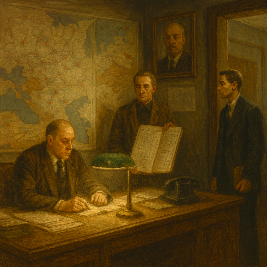
☭ Party Official (to Kantorovich): Wheat moves. Bread appears. Costs explode. Could you explain how the first two can occur without the third?

🧮 Kantorovich:
Hmm, it is the Monge’s French approach to optimal transport. This method allows only one-to-one assignments — a farm to a single factory. It is beautiful—like a court etiquette manual. It also breaks the budget when capacities don’t line up.

☭ Official: Examples?

🧮 Kantorovich: Farm A has 2 tons; Mill 1 and Mill 2 each need 1 ton.
Monge’s rule can’t split A—so either we overflow a mill or we ship the extra far away at great cost. It is time we shall stop assigning by etiquette and start assigning by fractions. One farm’s harvest may be shared among Leningrad, Moscow, and Kiev (several mills). No drama, no lace.

☭ Official (suspicious):
Shared? You propose to slice the wheat like bourgeois cake?

🧮 Kantorovich (calmly):
Not cake—convexity.

☭ Official: Could you explain your method. How do we schedule wheat to mills?

🧮 Kantorovich: We keep the same data: farms live in \(X\) with supply measure \(\mu\), mills live in \(Y\) with capacity measure \(\nu\), and \(c(x,y)\) is the per–unit haul cost. Normalize so \(\mu(X)=\nu(Y)=1).\)

We will not do a single address per farm, but a plan \(\pi\): it tells what fraction of wheat goes from each farm \(x\) to each mill \(y\).
Mathematically, \(\pi\) is a measure on \(X\times Y\) with the correct row and column totals (marginals):
\[\Pi(\mu,\nu):=\Big\{\pi\text{ on }X\times Y:\ \pi(A\times Y)=\mu(A),\ \ \pi(X\times B)=\nu(B)\ \ \forall A\in\mathcal B_X,\ B\in\mathcal B_Y\Big\}.\]

Spreadsheet intuition: rows = farms, columns = mills; the entry \(\pi(x,y)\) is the fraction shipped \(x\to y\).
Row sums match \(\mu\) (every farm ships all its wheat); column sums match \(\nu\) (every mill is filled exactly).

☭ Official: And we choose \(\pi\) how?

🧮 Kantorovich: By minimizing the national bill (the expected cost under \(\pi)\):

\[
\min_{\pi\in\Pi(\mu,\nu)} \ \int_{X\times Y} c(x,y)\,d\pi(x,y)\ \qquad \text{(mass may split).}\]

If the country’s total wheat is \(S\) tons (before normalization), the physical cost is \(S!\int c\,d\pi\).

☭ Official: Why is this reliable?

🧮 Kantorovich: Because the feasible set \(\Pi(\mu,\nu)\) is convex (mixtures of schedules are schedules) and the objective is linear in \(\pi\). On reasonable spaces \(Polish (X,Y)\) (e.g.\ subsets of \(\mathbb R^2\)) with a lower semicontinuous cost \(c\) (no sudden discounts), an optimal plan exists. Always.

☭ Official (nodding): Fractions in the boxes, rows = supply, columns = demand, minimize the sum. No lace.

🧮 Kantorovich (smiles): Exactly. More bread, fewer marathons.

☭ Official: And how do we know which roads actually carry wheat? I dislike paying for decorations.

🧮 Kantorovich: We use shadow prices. Assign a number to each farm and each mill:
\[
\varphi:X\to\mathbb R\quad(\text{farms}),\qquad \psi:Y\to\mathbb R\quad(\text{mills}),
\]
with the global no-underpricing rule
\[
\varphi(x)+\psi(y)\le c(x,y)\quad\text{for all }(x,y).
\]
Then we maximize the total value
\[
\sup_{\varphi,\psi}\ \Big(\int_X \varphi\,d\mu+\int_Y \psi\,d\nu\Big)\ \text{ subject to }\ \varphi+\psi\le c\ .
\]
Strong duality holds: this supremum equals the minimal transport cost. At the optimal schedule \(\pi^\ast\),
\[
\varphi^\ast(x)+\psi^\ast(y)=c(x,y)\quad\text{for }\pi^\ast\text{-a.e. }(x,y),
\]
so wheat flows only on tight routes. Overpriced routes carry no flow.

☭ Official: Good. Prices that turn lights on where grain should move. When do we get back to one arrow per farm?

🧮 Kantorovich: When nature is kind. If supply isn’t all concentrated at points and the cost rewards straight, nearby routes, the best schedule often behaves like a single address per source—effectively a map. But that conclusion belongs to future mathematics, Comrade; today we use the plan.

☭ Official: And what do the clerks actually compute while I frown at the portrait?

🧮 Kantorovich: A linear program. With farms \(i\), mills \(j\), shipments \(x_{ij}\ge0\), costs \(c_{ij}=c(x_i,y_j)\):
\[
\begin{aligned}
\min_{x_{ij}\ge0}\quad & \sum_{i,j} c_{ij}\,x_{ij} \
\text{s.t.}\quad & \sum_j x_{ij}=s_i\quad(\text{ship all supply}),\qquad
\sum_i x_{ij}=d_j\quad(\text{fill all mills}).
\end{aligned}
\]
Normalize by \(S=\sum_i s_i): (\pi_{ij}:=x_{ij}/S\) is a discrete coupling in \(\Pi(\mu,\nu)\) and
\(\sum c_{ij}x_{ij}=S\int c\,d\pi\).
They can solve it by transportation algorithms; your signature appears only at the end.

☭ Official(closing the file): Prices to light the roads, plans to split the loads, and arrows when the heavens permit. Acceptable.

🧮 Kantorovich(dry): Monge when you can, coupling when you must. Either way, warm bread—without marathons.

The clerk exhales. The portrait approves. The spreadsheet looks slightly less terrifying.

Act III — Paris, 1991

Scene: Seminar room; chalk dust in sunbeams. A blackboard already half-conquered. Enter Yann Brenier, chalk in hand. In the back row sit two ghosts: Monge (with a ruler) and Kantorovich (with a ledger).

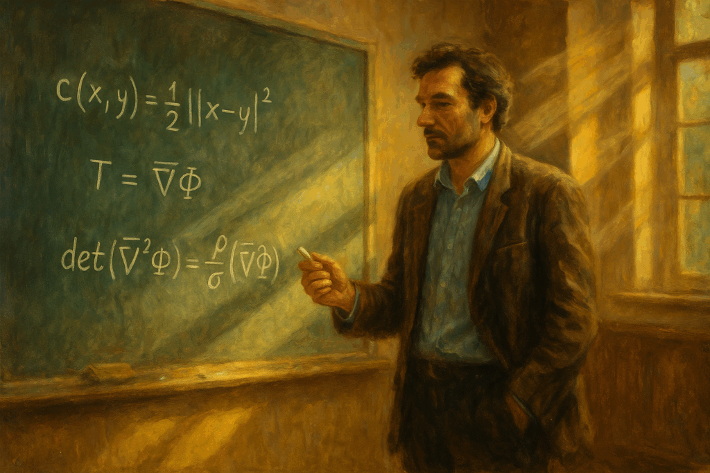
Brenier (calm, to the room): Suppose our cost is the squared distance,
\[
c(x,y)=\frac{1}{2}\|x-y\|^2,
\]
and the country’s wheat is not piled into atoms but spread with a density (i.e., \(\mu\) is absolutely continuous). Then the optimal transport is not merely a schedule—it is a map. More precisely:

Brenier’s Theorem (1991). Let \(\mu,\nu\) be probability measures on \(\mathbb{R}^d\) with finite second moments, and assume \(\mu\ll \mathrm{Leb}\) (no atoms). For \(c(x,y)=\tfrac12|x-y|^2\), there exists a (a.e.\ unique) optimal Monge map
\[
\boxed{\,T=\nabla \Phi\,}
\]
for some convex potential \(\Phi:\mathbb{R}^d\to\mathbb{R}\cup{+\infty}\), and the optimal plan is concentrated on its graph:
\[
\pi^\ast=(\mathrm{id},T)_{\#}\mu .
\]

1. Finite second moments: \(\int |x|^2\,d\mu(x)<\infty\) and \(\int |y|^2\,d\nu(y)<\infty\). This says the average squared distance of mass from the origin is finite (a finite “moment of inertia”). It guarantees that the quadratic transport cost \(\int \tfrac12|x-y|^2\,d\pi\) can be finite for some coupling \(\pi\).
2. Absolute continuity of \(\mu\): no single point of \(X\) carries positive mass. Physically, the supply is a density, not a pile of atoms. This prevents a point-mass from being forced to split and allows the optimal coupling to be given by a function \(T\) rather than a multivalued plan.
3. Quadratic cost: the geometry of \(\tfrac12|x-y|^2\) forces optimal couplings to be (c)-cyclically monotone; such sets are subdifferentials of convex functions. This is the mechanism that produces \(T=\nabla\Phi\).

Brenier (sketches gradient arrows): Think of \(\Phi\) as a convex landscape over the country. At location \(x\), the arrow \(\nabla\Phi(x)\) points “straight uphill.” My theorem says: for squared-distance cost and a smooth supply, the cheapest rearrangement sends each infinitesimal grain along these gradient arrows to its unique destination \(T(x)\). Convexity forbids cost-lowering cycles; gradients do not swirl.
Each farm-point \(x\) sends its infinitesimal mass along \(\nabla\Phi(x)\) to a unique mill \(T(x)\). No crossings, no marathons.

Monge (ghost, delighted): Une fl`eche par point. The arrows return!

🧮 Kantorovich (ghost, approving): Through a convex potential—my ledger smiles.

Consequences (when densities exist).
If \(\mu=\rho(x)\,dx\) and \(\nu=\sigma(y)\,dy\), then \(\Phi\) solves, in the weak (a.e.) sense, the Monge–Amp`ere equation
\[
\det\big(\nabla^2\Phi(x)\big)=\frac{\rho(x)}{\sigma\big(\nabla\Phi(x)\big)}\,,
\qquad\text{and}\qquad
T_{\#}\mu=\nu .
\]
The displacement interpolation
\[
\mu_t:=\big((1-t)\,\mathrm{id}+t\,T\big)_{\#}\mu,\qquad t\in[0,1],
\]
is a constant-speed geodesic in the 2-Wasserstein space \(W_2(\mathbb{R}^d)\) between \(\mu\) and \(\nu\).

Short answer to why.
Optimal couplings for the quadratic cost are (c)-cyclically monotone; Rockafellar’s theorem puts such sets inside the subdifferential \(\partial\Phi\) of a convex \(\Phi\). Absolute continuity of \(\mu\) makes \(\partial\Phi\) single-valued \(\mu\)-a.e., yielding \(T=\nabla\Phi\) (existence and uniqueness).

Brenier drops the chalk. The ghosts exchange a courteous bow: arrows for Louis XVI, convexity for the Bureau. Outside, somewhere, peasants are happy, and there is enough bread to feed the kingdom.

Acknowledgments. I’m grateful to professor Nestor Gullen, who introduced me to the main ideas of optimal transport during my time as a volunteer assistant on his Algorithms for Convex Surface Construction project. Many thanks to research fellows Stephanie Atherton; Matthew Hellinger; Minghao Ji; Amar KC; Marina Oliveira Levay Reis, for being a joy to work with—curious, rigorous, and creative, and to professor Justin Solomon as well for assigning me this project, and making SGI awesome.

Historical note & disclaimer

This tale is fictional. The conversations attributed to Louis XVI, Gaspard Monge, and Leonid Kantorovich are the product of the author’s imagination.

Bibliography

1. Introduction to Gradient Flows in the 2-Wasserstein Space | Abdul Fatir Ansari. (n.d.). Retrieved August 22, 2025, from https://abdulfatir.com/blog/2020/Gradient-Flows/
2. Frederic Schuller (Director). (2016, March 13). Measure Theory  -Lec05- Frederic Schuller [Video recording]. https://www.youtube.com/watch?v=6ad9V8gvyBQ
3. Monge, G. (1781). Mémoire sur la théorie des déblais et des remblais. Mem. Math. Phys. Acad. Royale Sci., 666–704.
4. Peyré, G. (2025). Optimal Transport for Machine Learners. arXiv Preprint arXiv:2505.06589.
5. Santambrogio, F. (n.d.). Optimal Transport for Applied Mathematicians – Calculus of Variations, PDEs and Modeling.