Differential geometry makes heavy use of calculus in order to study geometric objects such as smooth manifolds. Just as differential geometry builds upon calculus and other fundamentals, the notion of differential forms extend the approaches of differential geometry and calculus, even allowing us to study the larger class of surfaces that are not necessarily smooth. We will motivate from calculus a brief brush with differential forms and their geometric potential.
Review of Vector Fields
Recall a vector field is a special case of a multivariable vector-valued function (taking in a scalar or a vector and outputting a set of multidimensional vectors). Often they are defined in \(\mathbb{R}^2\) or \(\mathbb{R}^3\), but can also be defined more generally on smooth manifolds.
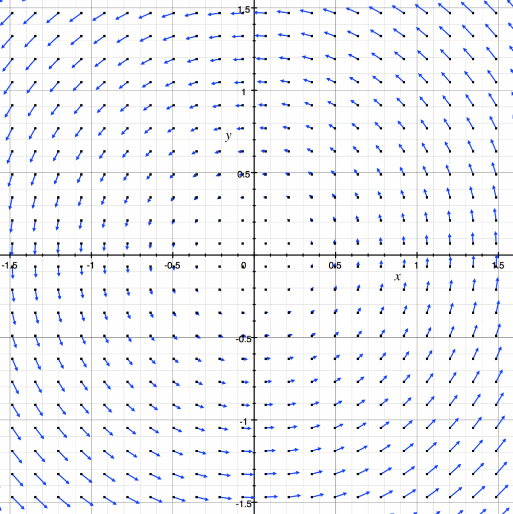
In three dimensional space, a vector field is a function \(V\) that assigns to each point \((x, y, z)\) a three dimensional vector given by \(V(x, y, z)\). Consider our identity function
$$ V(x, y, z) = \begin{bmatrix}x\\y\\z \end{bmatrix}, $$
where for each point \((x, y, z)\) we associate a vector with those same coordinates. Generalizing, for any vector function \(V(x, y, z)\), we visualize its vector field by placing the tail of the corresponding vector \(V(x_0, y_0, z_0)\) at its point \((x_0, y_0, z_0)\) in the domain of \(V(x, y, z)\).
Vector fields can be transformed into scalar fields via \(\nabla\) taken as a vector differentiable operator known as the gradient operator.
Our gradient points in the direction of steepest ascent of a scalar function \(f(x_1, x_2, x_3, . . . x_n)\), indicating the direction of greatest change of \(f\). A vector field \(V\) over an open set \(S\) is a gradient field if there exists a differentiable real-valued function (the scalar field) \(f\) on \(S\). Then
$$V = \nabla f = ( \frac{\partial f}{\partial x_1}, \frac{\partial f}{\partial x_2}, \frac{\partial f}{\partial x_3}, . . . \frac{\partial f}{\partial x_n})$$
is a special type of vector field \(V\) defined as the gradient of a scalar function, where each \( v \in V\) is the gradient of \(f\) at that point.
The Divergence and Curl Operators
Now that we have reviewed vector fields, recall that we can also perform operations like divergence and curl over them. When fluid flows over time, some regions of fluid will become less dense with particles as they flow away (negative divergence). Meanwhile, particles tending towards each other will cause the fluid in that region to be more dense (positive divergence).
Luckily, we have our handy divergence operator to take in the vector-valued function of our vector field and output a scalar-valued function measuring the change in density of the fluid around each point. Given a vector field \(V\), we can think of divergence
$$\text{div}\space V = \nabla \cdot V = \frac{\partial V_1}{\partial x} + \frac{\partial V_2}{\partial y}+ \frac{\partial V_3}{\partial z} . . . $$
as a variation of the derivative that generalizes to vector fields \(V\) of any dimension. Another “trick” to thinking about the divergence formula is as the trace of the Jacobian matrix of the vector field.
In differential geometry, one can also define divergence on a Riemannian manifold \((M, g)\), a smooth manifold \(M\) endowed with the Riemannian metric \(g\) as a choice of inner product for each tangent space of \(M\).

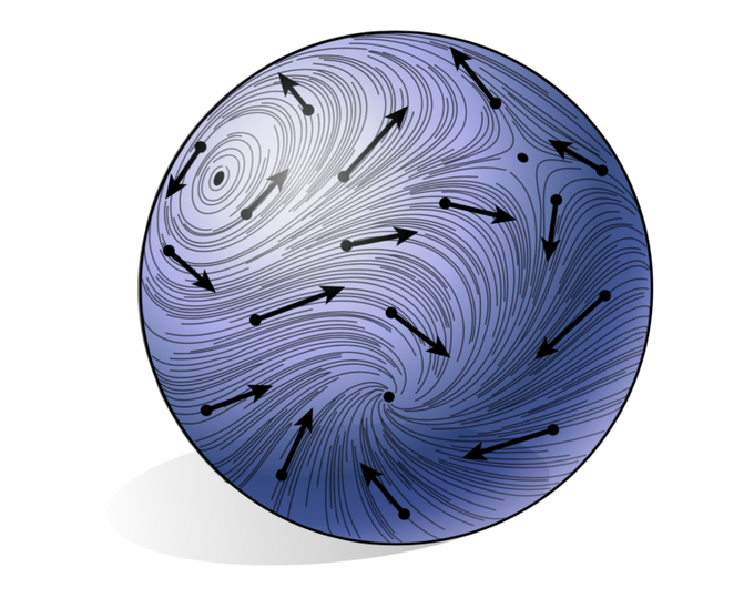
Whereas divergence describes changes in density, curl measures the “rotation”, or angular momentum, of the vector field \(V\). Likewise, the curl operator takes in a vector-valued function and outputs a function that describes the flow of rotation given by the vector field at each point.
For a vector field function
$$V(x, y) = v_1(x, y)\hat{i} + v_2(x, y)\hat{j},$$
we can look at the change of a point \((x_0, y_0)\) by looking at the change in \(v_1\) as \(y\) changes and \(v_2\) as \(x\) changes. We calculate
$$2\text{d curl} \space V = \nabla \times V = \frac{\partial v_2}{\partial x}(x_0, y_0) \space – \frac{\partial v_1}{y}(x_0, y_0),$$
with a positive evaluation indicating counterclockwise rotation around \((x_0, y_0)\) and a negative evaluation indicating clockwise.
Approach by Differential Forms
While curl is typically only defined in two and three dimensions, it can be generalized in the context of differential forms. The calculus of differential \(k\)-forms offers a unified approach to define integrands over curves, surfaces, and higher-dimensional manifolds. Differential 1-forms of expression form
$$\omega = f(x)dx$$
are defined on an open interval \( U \subseteq \mathbb{R^n}\) with \(f: U \to \mathbb{R}\) a smooth function. We can have 1-forms
$$\omega = f(x, y)dx + g(x, y)dy$$
defined on an open subset \( U \subseteq \mathbb{R^2}\) ,
$$\omega = f(x, y, z)dx + g(x, y, z)dy + h(x, y, z)dz $$
defined on an open subset \( U \subseteq \mathbb{R^3}\), and so on for any positive integer \(n\).
Correspondence Theorem: Given a 1-form \(\omega = f_1dx_1 + f_2dx_2 + . . . f_ndx_n\), we can define an associated vector field with component functions \((f_1, f_2, . . . f_n)\). Conversely, given a smooth vector field \(V = (f_1, f_2, . . . f_n)\), we can define an associated 1-form \(\omega = f_1dx_1 + f_2dx_2 + . . . f_ndx_n\).
Via the exterior derivative and an extension of the correspondence between 1-forms and vector fields to arbitrary \(k\)-forms, we can generalize the well-known operators of vector calculus.
The exterior derivative \(d\omega\) of a \(k\)-form is simply a \(k + 1\)-form. We provide an example of its use in defining curl:
Let \(\omega = f(x, y, z)dx + g(x, y, z)dy + h(x, y, z)dz\) be a 1-form on \( U \subseteq \mathbb{R}^3\) with its associated vector field \(V = (f, g, h)\). Its exterior derivative \(d\omega\) is the 2-form
$$d\omega = (\frac{\partial h}{\partial y} – \frac{\partial g}{\partial z}) dy \wedge dz + (\frac{\partial f}{\partial z} – \frac{\partial h}{\partial x}) dz \wedge dx + (\frac{\partial g}{\partial x} – \frac{\partial f}{\partial y}) dx \wedge dy,$$
where \(\wedge\) is an associative operation known as the exterior product. We define the curl of \(V\)
$$ \nabla \times V = (\frac{\partial h}{\partial y} – \frac{\partial g}{\partial z}), (\frac{\partial f}{\partial z} – \frac{\partial h}{\partial x}), (\frac{\partial g}{\partial x} – \frac{\partial f}{\partial y})$$
as the vector field associated to the 2-form \(d\omega\). Attempt to see how this definition of curl agrees with the traditional version, but can be applied in higher dimensions.
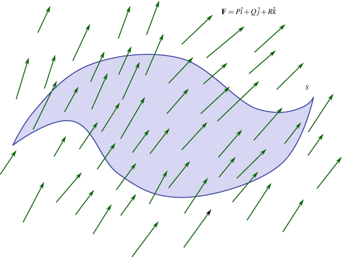
The natural pairing between vector fields and 1-forms allows for the modern approach of \(k\)-forms for multivariable calculus and has also heavily influenced the area of geometric measure theory (GMT), where we define currents as functionals on the space of \(k\)-forms. Via currents, we have the impressive result that a surface can be uniquely defined by the result of integrating differential forms over it. Further, the differential forms fundamental to GMT open up our toolbox to studying geometry that is not necessarily smooth!
Acknowledgements. We thank Professor Chien, Erick Jiminez Berumen, and Matheus Araujo for exposing us to new math, questions, and insights, as well as for their mentorship and dedication throughout the “Developing a Medial Axis for Measures” project. We also acknowledge Professor Solomon for suggesting edits incorporated into this post, as well as for his organization of the wonderful summer program in the first place!