SGI Fellows: Haojun Qiu, Nhu Tran, Renan Bomtempo, Shree Singhi and Tiago Trindade
Mentors: Sina Nabizadeh and Ishit Mehta
SGI Volunteer: Sara Samy
Introduction
The field of Computational Fluid Dynamics (CFD) has long been a cornerstone of both stunning visual effects in movies and video games, and also a critical tool in modern engineering, for designing more efficient cars and aircrafts for example.
At the heart of any CFD application there exists a solver that essentially predicts how a fluid moves in space at discrete time intervals. The dynamic behavior of a fluid is governed by a famous set of partial differential equations, called the Navier-Stokes equations, here presented in vector form:
$$
\begin{align}
\frac{\partial \mathbf{u}}{\partial t}
+ (\mathbf{u} \cdot \nabla) \mathbf{u} &=
-\frac{1}{\rho} \nabla p
+ \nu \nabla^{2} \mathbf{u}
+ \mathbf{f},
\quad
\text{subject to}\quad \nabla \cdot \mathbf{u}
&=
0,
\end{align}
$$
where \(t\) is time, \(\mathbf{u}\) is the varying velocity vector field, \(\rho\) is the fluids density, \(p\) is the pressure field, \(\nu\) is the kinematic viscosity coefficient and \(\mathbf{f}\) represents any external body forces (e.g. gravity, electromagnetic, etc.). Let’s quickly break down what each term means in the first equation, which describes the conservation of momentum:
- \(\dfrac{\partial \mathbf{u}}{\partial t}\) is the local acceleration, describing how the velocity of the fluid changes at a fixed point in space.
- \((\mathbf{u} \cdot \nabla) \mathbf{u}\) is the advection (or convection) term. It describes how the fluid’s momentum is carried along by its own flow. This non-linear term is the source of most of the complexity and chaotic behavior in fluids, like turbulence.
- \(\frac{1}{\rho}\nabla p\) is the pressure gradient. It’s the force that causes fluid to move from areas of high pressure to areas of low pressure.
- \(\nu \nabla^{2} \mathbf{u}\) is the viscosity or diffusion term. It accounts for the frictional forces within the fluid that resist flow and tend to smooth out sharp velocity changes. For the “Gaussian Fluids” paper, this term is ignored (\(\nu=0\)) to model an idealized inviscid fluid.
The second equation, \(\nabla \cdot \mathbf{u} = 0\), is the incompressibility constraint. It mathematically states that the fluid is divergence-free, meaning it cannot be compressed or expanded.
The first step to numerically solving these equations on some spatial domain \(\Omega\) using classical solvers is to discretize this domain. To do that, two main approaches have dominated the field from its very beginning:
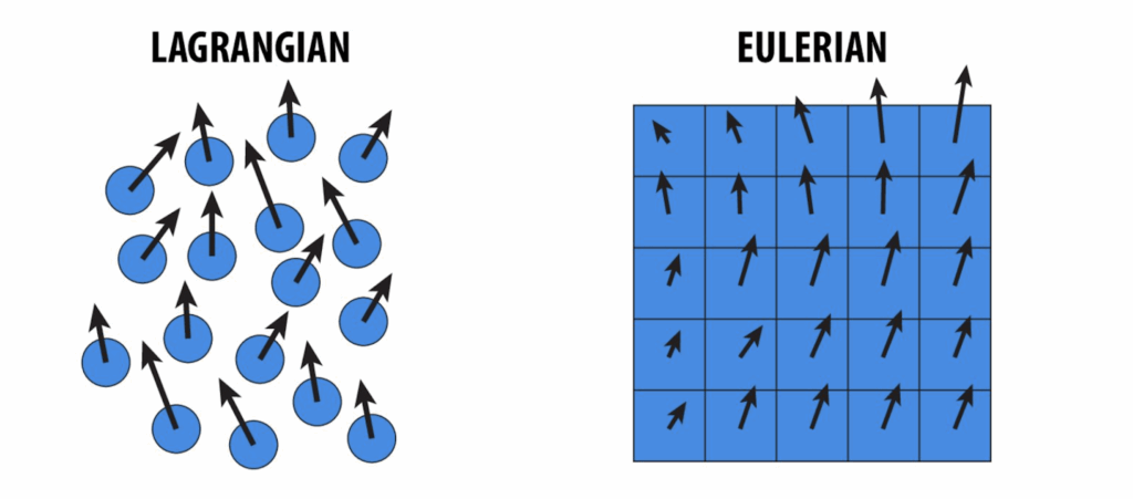
- Eulerian methods: which use fixed grids that partition the spatial domain into a (un)structured collection of cells on which the solution is approximated. However, these methods often suffer from “numerical viscosity,” an artificial damping that smooths away fine details;
- Lagrangian methods: which use particles to sample the solution at certain points in space and that move with the fluid flow. However, these methods can struggle with accuracy and capturing delicate solution structures.
The core problem has always been a trade-off. Achieving high detail with traditional solvers often requires a massive increase in memory and computational power, hitting the “curse of dimensionality”. Hybrid Lagrangian-Eulerian methods that try to combine the best of both worlds can introduce their own errors when transferring data between grids and particles. The quest has been for a representation that is expressive enough to capture the rich, chaotic nature of fluids without being computationally prohibitive.
A Novel Solution: Gaussian Spatial Representation
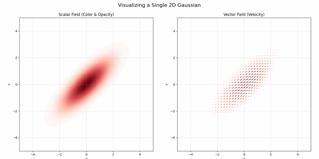
By now you have probably come across an emerging technology in the field of 3D rendering called 3D Gaussian Splatting (3DGS). It attempts to represent a 3D scene using, not traditional polygonal meshes or volumetric voxels, but in a manner similar to an artist using paint brush strokes to approximate a colored picture, Gaussian Splatting uses 3D gaussians to “paint” a 3D scene. These gaussians are nothing more than a ellipsoid with a color value and opacity associated.
Think of each Gaussian not as a solid, hard-edged ellipsoid, but as a soft, semi-transparent cloud (Fig.2). It’s most opaque and dense at its center and it smoothly fades to become more transparent as you move away from the center. The specific shape, size, and orientation of this “cloud” are controlled by its parameters. By blending thousands or even millions of these colored, transparent splats together, Gaussian Splatting can represent incredibly detailed and complex 3D scenes.
Drawing from this incredible effectiveness of using gaussians to encode complex geometry and lighting of 3D scenes, a new paper presented at SIGGRAPH 2025 titled “Gaussian Fluids: A Grid-Free Fluid Solver based on Gaussian Spatial Representation” by Jingrui Xing et al. introduces a fascinating new approach to computational domain representation for CFD applications.
The new method, named Gaussian Spatial Representation (GSR), uses gaussians to essentially “paint” vector fields. While 3DGS encodes local color information into each gaussian, GSR encodes local vector fields. In this way each gaussian stores a vector that defines a local direction of the velocity field, where the magnitude of the vectors is greater closer the gaussian’s center, and quickly gets smaller when moving farther from it. In Fig.2 we can see an example of 2D gaussian viewed with color data (left), as well as with a vector field (right).
By splatting a lot of these gaussians and adding the vectors we can then define a continuously differentiable vector field around a given domain, which allows us to solve the complex Navier-Stokes equations not through traditional discretization, but as a physics-based optimization problem at each time step. A custom loss function ensures the simulation adheres to physical laws like incompressibility (zero-divergence) and, crucially, preserves the swirling motion (vorticity) that gives fluids their character.
Enforcing Physics Through Optimization: The Loss Functions
The core of the “Gaussian Fluids” method is its departure from traditional time-stepping schemes. Instead of discretizing the Navier-Stokes equations directly, the authors reframe the temporal evolution of the fluid as an optimization problem. At each time step, the solver seeks to find the set of Gaussian parameters that best satisfies the governing physical laws. This is achieved by minimizing a composite loss function, which is a weighted sum of several terms, each designed to enforce a specific physical principle or ensure numerical stability.
Two of the main loss terms are:
- Vorticity Loss (\(L_{vor}\)): For a two dimensional ideal (inviscid) fluid, vorticity, defined as the curl of the velocity field (\(\omega=\nabla \times u\)), is a conserved quantity that is transported with the flow. This loss function is designed to uphold this principle. It quantifies the error between the vorticity of the current velocity field and the target vorticity field, which has been advected from the previous time step. By minimizing this term, the solver actively preserves the rotational and swirling structures within the fluid. This is critical for preventing the numerical dissipation (an artificial smoothing of details) that often plagues grid-based methods and for capturing the fine, filament-like features of turbulent flows.
- Divergence Loss (\(L_{div}\)): This term enforces the incompressibility constraint, \(\nabla \cdot u=0\). From a physical standpoint, this condition ensures that the fluid’s density remains constant; it cannot be locally created, destroyed, or compressed. The loss function achieves this by evaluating the divergence of the Gaussian-represented velocity field at numerous sample points and penalizing any non-zero values. Minimizing this term is essential for ensuring the conservation of mass and producing realistic fluid motion.
Beyond these two, to function as a practical solver, the system must also handle interactions with boundaries and maintain stability over long simulations. The following loss terms address these requirements:
- Boundary Losses (\(L_{b1}\), \(L_{b2}\)): The behavior of a fluid is critically dependent on its interaction with solid boundaries. These loss terms enforce such conditions. By sampling points on the surfaces of geometries within the scene, the loss function penalizes any fluid velocity that violates the specified boundary conditions. This can include “no-slip” conditions (where the fluid velocity matches the surface velocity, typically zero) or “free-slip” conditions (where the fluid can move tangentially to the surface but not penetrate it). This sampling-based strategy provides an elegant way to handle complex geometries without the need for intricate grid-cutting or meshing procedures.
- Regularization Losses (\(L_{pos}\), \(L_{aniso}\), \(L_{vol}\)): These terms are included to ensure the numerical stability and well-posedness of the optimization problem.
- The Position Penalty (\(L_{pos}\)) constrains the centers of the Gaussians, preventing them from deviating excessively from the positions predicted by the initial advection step. This regularizes the optimization process, improves temporal coherence, and helps prevent particle clustering.
- The Anisotropy (\(L_{aniso}\)) and Volume (\(L_{vol}\)) losses act as geometric constraints on the Gaussian basis functions themselves. They penalize Gaussians that become overly elongated, stretched, or distorted. This is crucial for maintaining a high-quality spatial representation and preventing the numerical instabilities that could arise from ill-conditioned Gaussian kernels.
However, when formulating a fluid simulation as a Physics-Based optimization problem, one challenge that soon becomes apparent is that choosing good loss functions can be really tricky. The reliance on “soft constraints”, such as the divergence loss function, in the optimization process means that small errors can accumulate over time. Also, the handling of complex domains with holes (non-simply connected domains) is also a big challenge.
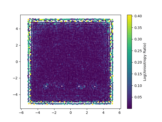
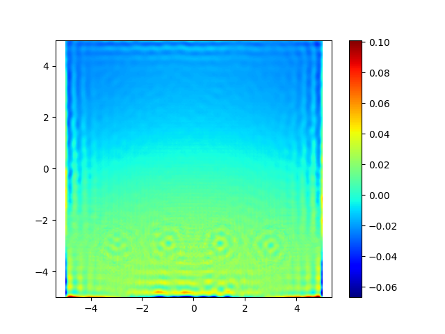
When running the Leapfrog simulation we can see that the divergence of the solution, although relatively small, isn’t as close to zero as it should be (ideally it should be exactly zero).
Divergence-free Gaussian Representation
Now we want to extend on this paper a bit. Let’s focus on the 2D case for now. The problem of regularizing divergence is that the velocity vector field won’t be exactly divergence free. I can perhaps help this with an extra step every iteration. Define \(\mathbf{J} \in \mathbb{R}^{2 \times 2}\) as a rotation matrix
$$
\mathbf{J} = \begin{bmatrix}
0 & -1\\
1 & 0
\end{bmatrix}.
$$
It is known that for any potential function \(\phi: \mathbb{R}^{2} \to \mathbb{R}\), we have \(\mathbf{J} \ \nabla\phi(\mathbf{x})\) divergence free:
$$
\nabla \cdot (\mathbf{J} \ \nabla \phi) = –
\frac{\partial }{\partial x} \frac{\partial \phi}{ \partial y} + \frac{\partial}{\partial y} \frac{\partial \phi}{\partial x} = 0.
$$
This potential function can be constructed with the same gaussian mixture by carrying a \(\phi_{i} \in \mathbb{R}\) at every gaussian, and thus a continuous function having full support
$$
\phi(\mathbf{x}) = \sum_{i=1}^{N} \phi_i G_i(\mathbf{x}).
$$
similarly we can replace \(G_i(\mathbf{x})\) with the clamped gaussians \(\tilde{G}_i(\mathbf{x})\) for efficiency. Now we can construct a vector field that is unconditionally divergence-free
$$
\mathbf{u}_{\phi}(\mathbf{x}) = \mathbf{J} \ \nabla \phi(\mathbf{x})
$$
and the gradient of the potential can be computed
$$
\begin{align}
\nabla \phi(\mathbf{x}) &= \sum_{i=1}^{N} \phi_i \nabla G_i(\mathbf{x}) \\
&= – \sum_{i=1}^{N} \phi_i G_i(\mathbf{x})
\mathbf{\Sigma}_{i}^{-1}
(\mathbf{x} – \mathbf{\mu}_i).
\end{align}
$$
so the equation can be written as
$$
\mathbf{u}_{\phi}(\mathbf{x})
= \sum_{i=1}^{N}
\underbrace{\left(
– \phi_i \mathbf{J} \mathbf{\Sigma}_{i}^{-1}(\mathbf{x} – \mathbf{\mu}_i)
\right)}_{\text{per-gaussian vector}}
G_i(\mathbf{x})
$$
We want to somehow fit this \(\mathbf{u}_{\phi}(\mathbf{x})\) to the vector field \(\mathbf{u}(x)\) directly from the gaussian velocities
$$
\mathbf{u}(\mathbf{x}) = \sum_{i=1}^{N} \mathbf{u}_i G_i(\mathbf{x}).
$$
This can be a simple loss
$$
\underset{\{\phi_i\}_{i=1}^{N}}{\arg\min} \frac{1}{d|\mathcal{D}|}
\int_{\mathcal{D}}
\|\mathbf{u}(\mathbf{x}) – \mathbf{J} \ \nabla \phi(\mathbf{x}) \|_{2}^{2}
\ \mathrm{d}\mathbf{x}
$$
and we use the similar approach of Monte Carlo way of sampling \(\mathbf{x}\) uniformly in space.
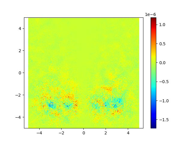
Doing this, we managed to achieve a divergence much closer to zero, as shown in the image below.
References
Jingrui Xing, Bin Wang, Mengyu Chu, and Baoquan Chen. 2025. Gaussian Fluids: A Grid-Free Fluid Solver based on Gaussian Spatial Representation. In Proceedings of the Special Interest Group on Computer Graphics and Interactive Techniques Conference Conference Papers (SIGGRAPH Conference Papers ’25). Association for Computing Machinery, New York, NY, USA, Article 9, 1–11. https://doi.org/10.1145/3721238.3730620