Project Mentor: Bailey Miller
1 Introduction
A classic problem in computer graphics is the interpolation of boundary values into a region’s interior. More formally, given a domain \( \Omega \) and values prescribed on its boundary \( \partial \Omega \), we seek a smooth function \( u: \mathbb{R}^n \to \mathbb{R} \) that satisfies the boundary value problem
$$\begin{align}
\Delta u(x) = 0 \text{ in } \Omega, \
\quad u(x) = g(x) \text{ on } \partial \Omega,
\end{align}$$
where \(g(x)\) is a given boundary function. This is the well-known Laplace’s equation with Dirichlet boundary conditions. A standard approach for solving such PDEs is the finite element method (FEM), which discretizes the domain into a mesh and computes a weak solution. However, the accuracy of FEM depends critically on the quality of the mesh and how well it approximates the domain geometry. In contrast, Monte Carlo methods offer an appealing alternative — particularly the walk on spheres (WoS) algorithm [Muller, 1956], which avoids meshing altogether. WoS exploits the Mean Value Property of harmonic functions (i.e., functions satisfying \( \Delta u = 0) \), which states:
$$\begin{align}
u(x) = \frac{1}{|\partial B(x, r)|} \int_{\partial B(x, r)} u(y) \ \mathrm{d}y,
\end{align} \quad \text{(*)}$$
for any ball \( B(x, r) \subseteq \Omega \). This property implies that \( u(x) \) can be estimated by recursively sampling points on the boundary of spheres centered at \( x \), continuing until a point lands on \( \partial \Omega \), where the value is known from \( g(x) \). Compared to FEM, WoS scales much better with geometric complexity and does not require certain properties of the mesh like watertightness, free of self-intersections, manifoldness, etc. While WoS does not generalize to all classes of PDEs, it offers many advantages even beyond geometric robustness (See Sawhney and Crane 2020, Section 1).
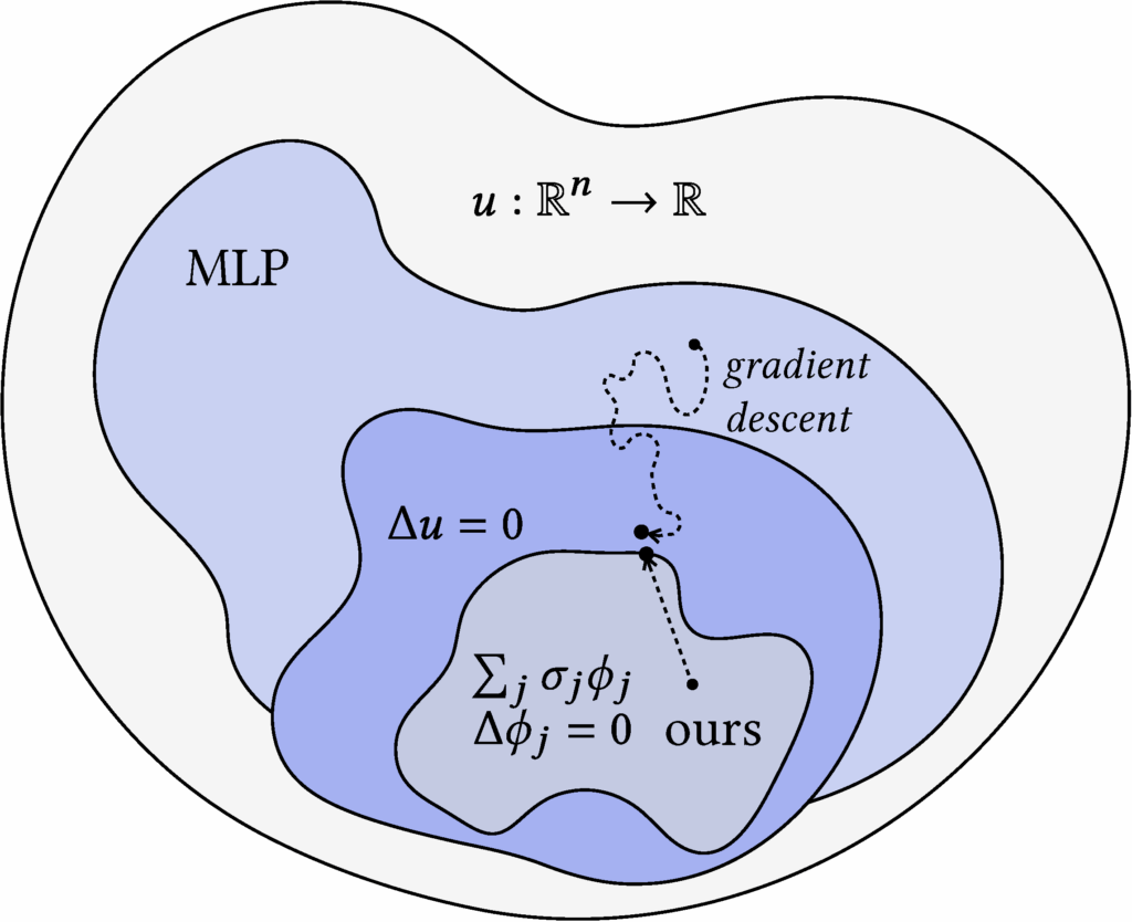
While WoS is an unbiased estimator and is largely agnostic to geometric quality, it can suffer from high variance, often requiring many samples to converge and thus incurring high computational cost. A common way to reduce variance is to use a control variate, and prior work has explored applying them to WoS. The main challenge in using control variates is finding a suitable reference function (one with a known integral) that also closely matches the target function. One research direction to address this challenge is neural control variates—constructing the control variate function using neural networks (See Li et al. 2024, who applied this approach to WoS). While their method leverages a clever technique known as automatic integration [Li et al. 2024] to perform closed-form integration, it still suffers from substantial overhead during both training and inference due to the use of MLPs. In contrast, we propose harmonic control variates, where harmonicity is built into the control variate representation by design, enabling closed-form integration directly as a function evaluation. Moreover, our representation is fitted using a simple least squares procedure, which is significantly more efficient than training a neural network via gradient descent. It also allows for much faster evaluation at inference time.
Specifically, our approach consists of two main steps. (1) We construct a harmonic representation as a weighted sum of harmonic kernels (e.g., Green’s functions), and fit the weights/coefficients using a sparse set of points in the domain along with their WoS-based estimates. This fitting reduces to solving a linear system of the form \( \Phi \sigma = u \) for the weight vector \( \sigma \). The resulting function is harmonic by construction, and although it provides a useful denoised estimate, it remains biased with respect to the true solution \( u(x) \) almost everywhere in the domain. (2) To correct for this bias, we use the harmonic representation as a control variate, thus termed harmonic control variate. Because the representation is harmonic, its mean over any sphere can be computed in closed form via simple function evaluation. We then define a residual Laplace problem, where the boundary condition is the difference between the true boundary data and our representation. Solving this residual problem with WoS and adding the result back to the harmonic representation yields an unbiased estimator for \( u(x) \). This control variate estimator reduces variance whenever the representation closely approximates \( u(x) \) on the boundary.
Our harmonic control variate achieves significant variance reduction compared to naive WoS across a range of geometries, yielding an average 40% reduction in RMSE compared to the naive baseline at 128 walks. In addition to its effectiveness, our method is simple to implement: the entire pipeline can be reproduced in Python with minimal code, leveraging just a few function calls to the underlying integrated C++ library Zombie [Sawhney and Miller 2023]. To illustrate its flexibility, we also extend our approach to settings with Neumann boundary conditions and with an alternative Monte Carlo scheme Walk on Stars [Sawhney, Miller, et al. 2023]. We believe that this classically inspired yet practical control variate representation (a sum of harmonic kernels) offers useful insights for the broader computational science and graphics communities.
2 Background
2.1 Walk on Spheres
The Walk on Spheres (WoS) algorithm [Muller 1956] can be motivated in two complementary ways. One is via Kakutani’s principle, which states that the solution value \( u(x) \) of a harmonic function at any point \( x \in \Omega \) is equal to the expected boundary value \( u(x) = \mathbb{E}[g(y)] \), where \( y \in \partial \Omega \) is the first boundary point reached by a Brownian motion starting at \( x \). We focus on a second, more constructive motivation coming from the mean value property of harmonic functions (see eq. (*)). This property immediately suggests a single-sample Monte Carlo estimator:
$$\begin{align}
\langle u(x) \rangle = u(y),
\quad y \sim \mathscr{U}(\partial B(x,r)),
\end{align}$$
where \( \mathscr{U}(\partial B(x,r)) \) denotes the uniform distribution on the sphere of radius \( r \) centered at \( x \). Specifically, the mean value property suggests that this estimator is unbiased:
$$ \begin{align}
\mathbb{E}[\langle u(x) \rangle]
\,=\, \mathbb{E}_{y \sim \mathscr{U}(\partial B(x,r))}[u(y)] \,=\, \int_{\partial B(x,r)} p(y) u(y) \,\mathrm{d}y
\,=\, \frac{1}{|\partial B(x,r)|}\int_{\partial B(x,r)} u(y) \,\mathrm{d}y
\,=\, u(x),
\end{align} $$
where \( p(y) = 1/|\partial B(x,r)| \) denotes the uniform probability density on \( \partial B(x, r) \).
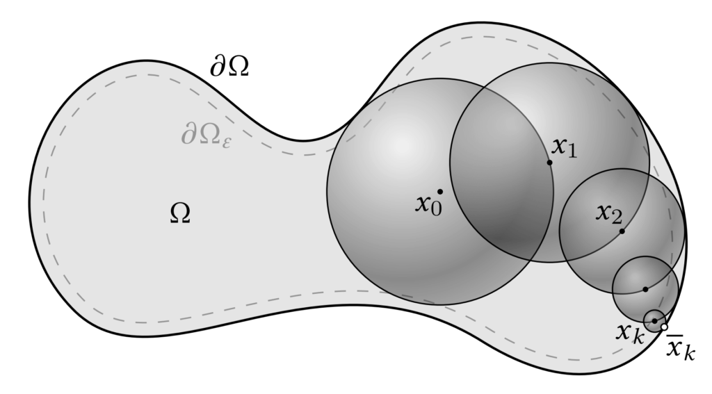
However, the difficulty is that \( u(y) \) is unknown unless \( y \) lies on the boundary \( \partial \Omega \). To address this, the mean value property is applied recursively: each sampled point becomes the new center for the next sphere, and the process continues until the boundary is reached. Since naïve recursion would never terminate, the algorithm introduces a tolerance \( \epsilon \). Specifically, once a point \( x_k \) lies within distance \( \epsilon \) of the boundary, we project it to the nearest boundary point \( \bar{x}_k \in \partial \Omega \) and evaluate the boundary condition \( g(\bar{x}_k) \). This serves as the base case of the recursion.
Formally, letting \( \Omega_\epsilon \) denote the \( \epsilon\)-shell adjacent to the boundary (illustrated in Figure 3), the recursive rule is
$$\begin{align}
\langle u(x_k) \rangle =
\begin{cases}
g(\bar{x}_k), & x_k \in \Omega\epsilon, \\
u(x_{k+1}), & \text{otherwise},
\end{cases}
\end{align}$$
with the next sample \( x_{k+1} \sim \mathscr{U}(\partial B(x_k, r_k)) \), where \( r_k \) is the largest radius such that the ball remains fully contained in \( \Omega \). As the recursion telescopes, the final estimator is simply
$$\begin{align}
\langle u(x_0) \rangle = g (\bar{x}_{n_i}^{(i)}), \quad x_n \in \Omega_{\epsilon},
\end{align}$$
where \( \bar{x}_n \) is the projected boundary point at termination.
By performing \( N \) independent walks and averaging their outcomes, we obtain a multi-sample Monte Carlo estimator of the solution:
$$\begin{align}
\langle u(x_0) \rangle_N = \frac{1}{N} \sum_{i=1}^N g\left( \bar{x}_{n_i}^{(i)}\right),
\end{align}$$
where each \( \bar{x}_{n_i}^{(i)} \in \partial \Omega \) is the endpoint of the \( i \)-th walk, reached on its \( n_i \)-th step. This estimator remains unbiased as \( \epsilon \to 0 \), but its efficiency is governed by the variance of the boundary condition \( g(x) \). In fact, the variance of the estimator is directly proportional to that of \( g(x) \):
$$\begin{align}
\mathrm{Var}[\langle u(x_0) \rangle_N]
= \frac{1}{N}\,\mathrm{Var}\left[g\left(\bar{x}_{n_i}^{(i)}\right)\right].
\end{align}$$
Intuitively, if \( g(x) \) varies significantly across the boundary region where walks terminate, the estimates \( \langle u(x_0) \rangle \) will fluctuate sharply between different exit points, leading to a noisy approximation of the solution. Conversely, if \( g(x) \) is nearly constant around the relevant boundary region, most walks yield similar values, and the estimator stabilizes. This observation is central to our two-pass variance-reduction strategy (see Section 3.2).
2.2 Control Variates
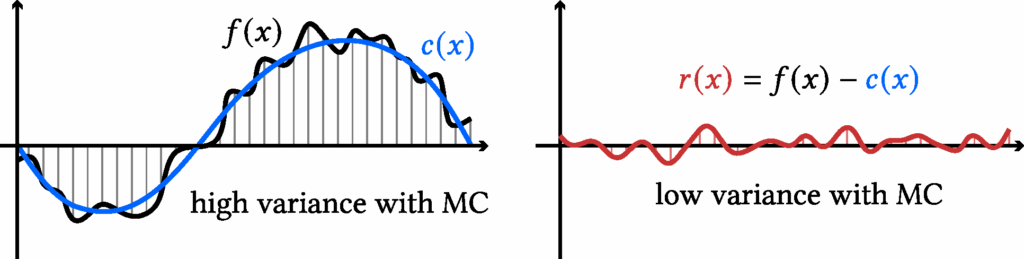
To build intuition, let us first consider the simple task of integrating a scalar function in one dimension. Suppose we want to estimate
$$\begin{align}
F = \int_{a}^{b} f(x)\, \mathrm{d}x,
\end{align}$$
using Monte Carlo (MC) sampling. A naive single-sample Monte Carlo estimator is
$$\begin{align}
\langle F \rangle = |b-a|\, f(x), \quad x \sim \mathscr{U}[a,b].
\end{align}$$
The idea of a control variate is to introduce a function (c(x)) that (i) closely approximates (f(x)) and (ii) has a known closed-form integral, denoted (C). We can rewrite the target integral as
$$\begin{align}
F = \int_a^b c(x)\, \mathrm{d}x + \int_a^b f(x) – c(x) \, \mathrm{d}x
= C + \int_a^b f(x) – c(x) \, \mathrm{d}x.
\end{align}$$
This yields a single sample Monte-Carlo estimator with control variate:
$$\begin{align}
\langle F \rangle^{(\text{cv})} = |b-a| \big(f(x) – c(x)\big) + C, \quad x \sim \mathscr{U}[a,b].
\end{align}$$
It is clear that it remains unbiased. Moreover, it achieves lower variance whenever the residual \( r(x) := f(x) – c(x) \) is less variable than the original function \( f(x) \):
$$\begin{align}
\mathrm{Var} [\langle F \rangle^{(\text{cv})} ]
<
\mathrm{Var}[\langle F \rangle]
\quad \iff \quad
\mathrm{Var}[f(x) – c(x)] < \mathrm{Var}[f(x)].
\end{align}$$
Control Variates for Walk-on-Spheres. Motivated by this principle, prior work [Li et al. 2024] incorporated control variates directly into the mean value formulation of WoS. At each step of the walk, they replace the boundary condition with a residual correction, and by eq. (*),
$$\begin{align} u(x) = \frac{1}{\lvert \partial B(x,r)\rvert}\int_{\partial B(x,r)} c(y)\,\mathrm{d}y + \frac{1}{\lvert \partial B(x,r)\rvert}\int_{\partial B(x,r)} \big(u(y)-c(y)\big)\,\mathrm{d}y \end{align}$$
where \( C(x) = \frac{1}{\lvert \partial B(x,r)\rvert}\int_{\partial B(x,r)} c(y)\,\mathrm{d}y \) and \( c : \mathbb{R}^d \to \mathbb{R} \) is the control variate. This introduces the challenge of designing a control variate \(c\) that is both expressive and admits a tractable integral \(C(x)\). Li et al. [2024] addressed this by parameterizing \( c \) with a neural network and using automatic integration to evaluate \(C(x)\). However, this approach requires costly neural network evaluations at every step of the walk and additional training via gradient descent. In contrast, we take the insight that if \( c \) is also harmonic, then \( C(x) = c(x) \) by eq. (*). Our method only evaluates the control variate twice per walk and fits it directly via least squares, making it significantly more efficient while still achieving variance reduction.
3 Method
Our method introduces a harmonic representation that serves as a control variate for variance reduction. We first describe the formulation of this harmonic representation and how it can be efficiently solved in Section 3.1. Next, we explain how this representation functions as a control variate to reduce variance in Monte Carlo estimation in Section 3.2. Finally, we present implementation details in Section 3.3. An overview of our method is illustrated in Figure 5.
3.1 Mixture of Harmonic Kernels Representation
We propose a simple, kernel-based representation for approximating a target harmonic function \( u(x) \), subject to Dirichlet boundary conditions \( u(x) = g(x) \) on \( \partial \Omega \). Specifically, we approximate \( u(x) \) using a mixture of harmonic kernels \( \phi_j(\,\cdot\,) \):
$$\begin{align}
c(x) = \sum_{j=1}^{M} \sigma_j \,\phi_j(x),
\end{align}$$
where each \( \phi_j(x) \) is itself harmonic. By linearity, the mixture \( c(x) \) is also harmonic. To ensure that \( c(x) \) remains free of singularities inside the domain \( \Omega \), the kernels are chosen carefully. The coefficients \( \{\sigma_j\}_{j=1}^M \) are free parameters that must be fitted to approximate \( u(x) \).
There are many possible choices of harmonic kernels. A canonical example in two dimensions is the Green’s function,
$$\begin{align}
\phi_j(x) = G^{\mathbb{R}^2}(x, y_j) = \frac{1}{2\pi} \log\bigl(\|x – y_j\|_2\bigr),
\end{align}$$
where the centers \( \{y_j\} \) are placed outside of \( \Omega \) to avoid singularities within the domain. We will introduce another kernel choice in Section 4.
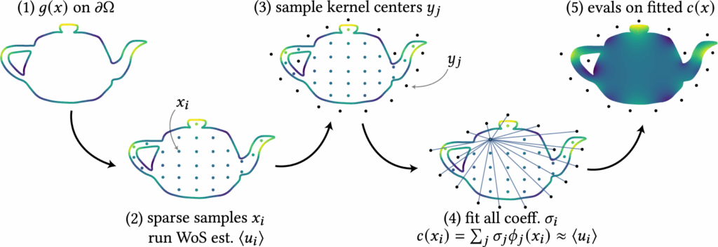
Fitting the coefficients: To determine the coefficients \( \sigma_j \), we first sample a sparse set of interior points \( \{x_i\}_{i=1}^N \subset \Omega \). At each point, we estimate \( \langle u(x_i) \rangle \) using Walk-on-Spheres (WoS), which leverages the known boundary condition. This produces training tuples \( \{(x_i, \langle u(x_i) \rangle) \}_{i=1}^N \), where \( c(x_i) \) should approximate \( \langle u(x_i) \rangle \). Each tuple gives a linear constraint on \( \sigma_j \), leading to the linear system:
\begin{bmatrix}
\phi_1(x_1) & \phi_2(x_1) & \cdots & \phi_M(x_1) \\
\phi_1(x_2) & \phi_2(x_2) & \cdots & \phi_M(x_2) \\
\vdots & \vdots & \ddots & \vdots \\
\phi_1(x_N) & \phi_2(x_N) & \cdots & \phi_M(x_N)
\end{bmatrix}
\begin{bmatrix}
\sigma_1 \\
\sigma_2 \\
\vdots \\
\sigma_M
\end{bmatrix}
=
\begin{bmatrix}
\langle u(x_1)\rangle \\
\langle u(x_2)\rangle \\
\vdots \\
\langle u(x_N)\rangle
\end{bmatrix} \quad \text{(**)}
\)
Solving this system yields the optimal coefficients {\( \sigma_j \)}. This can also be written as an optimization problem (the least square problem):
$$\begin{align}
\underset{\sigma \in \mathbb{R}^{M}}{\mathrm{argmin}} \,
\|\Phi \sigma – \langle u \rangle \|_{2}^{2},
\label{eq:optimize_lin_sys} \quad \text{(***)}
\end{align}$$
such that we can introduce some regularization terms (see Section 3.3). An example of this fitting procedure using the Green’s kernel is illustrated in Figure 6.
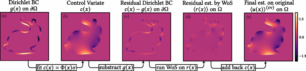
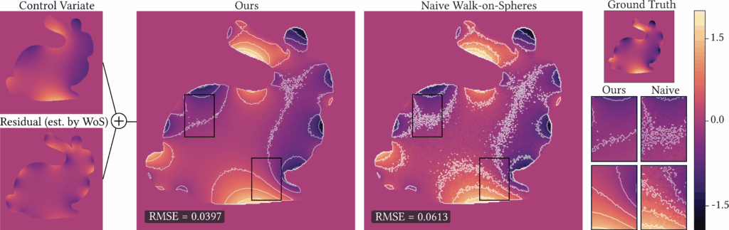
Intuitively, this representation projects the set of sparse and noisy estimates of \( u(x_i) \), i.e., the vector \( \langle u \rangle \), onto the subspace spanned by the harmonic kernels \( \{\phi_j(x)\} \). Since this fit is based only on a limited set of points and kernels and does not enforce correctness elsewhere, this representation is a biased estimator. Therefore, while this representation \( c(x) \) serves as a useful denoiser due to the smoothness of the kernels, it is not a sufficiently accurate approximation of the true solution \( u(x) \), see Figure 5. In the next section, we show how it can be leveraged as a control variate to reduce variance and obtain an unbiased estimate of \( u(x) \) throughout \( \Omega \).
3.2 Two-Pass with Control Variates
The main advantage of our representation \( c(x) \) being harmonic is that it satisfies \( \Delta c(x) = 0 \) in \( \Omega \). This allows us to define a residual PDE:
$$\begin{align}
\Delta\left[ u(x) – c(x) \right] = 0 \text{ in } \Omega, \
\quad u(x) – c(x) = g(x) – c(x) \text{ on } \partial \Omega,
\end{align}$$
which corresponds to solving for the harmonic residual function \( r(x) := u(x) – c(x)\). Since the Dirichlet boundary condition for \( r(x) \) is known, namely \( r(x) = g(x) – c(x) \) on \( \partial \Omega \), we can apply the Walk-on-Spheres (WoS) algorithm to estimate \( \langle r(x) \rangle \). Our control variate estimator for \( u(x) \) is then given by
$$\begin{align}
\langle u(x) \rangle^{(\text{cv})}
:= c(x) + \langle r(x) \rangle.
\end{align}$$
The argument for why this estimator is still unbiased and has smaller variance is similar to the 1D case outlined in Section 2.2. This estimator is unbiased since
$$\begin{align}
\mathbb{E}[\langle u(x) \rangle^{(\text{cv})}]
= \mathbb{E}[c(x) + \langle r(x) \rangle]
= c(x) + \mathbb{E}[\langle r(x) \rangle]
= c(x) + r(x)
= u(x),
\end{align}$$
where we used the fact that \( \mathbb{E}[\langle r(x) \rangle] = r(x) \) due to the unbiasedness of WoS. Therefore, as the number of random walks increases, the control variate estimator \( \langle u(x) \rangle^{(\text{cv})} \) converges to the true solution \( u(x) \). For variance reduction, observe that
$$\begin{align}
\mathrm{Var}[\langle u(x) \rangle^{(\text{cv})}]
= \mathrm{Var}[c(x) + \langle r(x) \rangle]
= \mathrm{Var}[\langle r(x) \rangle],
\end{align}$$
since \( c(x) \) is deterministic. Thus, we have:
$$\begin{align}
\mathrm{Var}[\langle u(x) \rangle^{(\text{cv})}] < \mathrm{Var}[\langle u(x) \rangle]
\quad \text{iff} \quad
\mathrm{Var}[\langle r(x) \rangle] < \mathrm{Var}[\langle u(x) \rangle].
\end{align}$$
As discussed earlier in the end of Section 2.1, variance is reduced when \( c(x) \) provides a good approximation to \( u(x) \) on the boundary. In this case, the residual boundary condition \( g(x) – c(x) \) has a smaller range, resulting in reduced variance in the WoS estimates for \( r(x) \) and, by extension, for \( u(x) \).
3.3 Implementation Details
We next describe several implementation choices in setting up and solving the linear system, as well as in implementing control variates.
Linear System Setup. Our formulation yields an \( N \times M \) linear system, where \( N \) is the number of constraints (sampled interior points) and \( M \) is the number of kernels. We deliberately set \( N > M \), making the system over-constrained. This avoids ill-posedness and eliminates the possibility of infinitely many solutions. To further enhance stability, we adopt Kd-tree based adaptive sampling, which distributes interior points evenly across the domain rather than allowing clusters in small regions. This reduces the risk of nearly colinear rows in the system matrix, which would otherwise harm numerical conditioning. Finally, we add regularization to eq. (***) to improve robustness near the boundary. Without it, the fitted representation tends to produce large coefficient magnitudes, leading to spikes and non-smooth artifacts. We experimented with both \( \ell_2 \) (ridge) regularization, which discourages large weights, and \( \ell_1 \) (lasso) regularization, which can additionally drive coefficients to zero. Both were effective, but we ultimately used \( \ell_2 \) in our experiments.
Control Variates with Zombie [Sawhney and Miller 2023]. We build on the Zombie library, which provides efficient C++ implementations of Monte Carlo geometry processing methods along with Python bindings. In the baseline setting, Zombie takes as input the geometry together with boundary conditions sampled on a grid. During Walk-on-Spheres (WoS), Zombie interpolates these grid values whenever a trajectory hits the boundary, and then outputs estimated interior values on a user-specified grid resolution. Our variance reduction technique using control variates requires only a minimal change to this setup. Instead of supplying the original boundary condition, we provide the boundary condition of the residual function. Zombie then performs WoS to estimate the residual inside the domain. The final solution is obtained by simply adding back the evaluation of \( c(x) \) on the grid to these residual estimates. This simple modification makes the method straightforward to implement while still delivering effective variance reduction.
4 Experiments
We explore two types of harmonic kernels for our harmonic representation. The first is the 2D fundamental solution (Green’s function): for \( x,y\in\mathbb{R}^2 \),
$$
\begin{align}
G^{\mathbb{R}^2}(x,y)=\frac{1}{2\pi}\log\|x-y\|_2,
\end{align}
$$
which satisfies \( \Delta_x G^{\mathbb{R}^2}(x,y)=\delta(x-y)\) and thus harmonic in \(x\) away from the singularity at \(y\); it underlies methods such as the Mixture of Fundamental Solutions and boundary-element approaches.
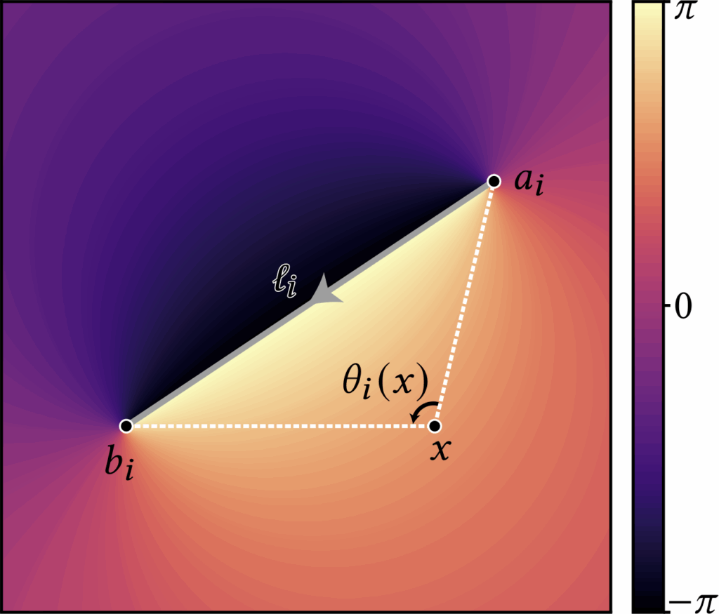
The second is the angle kernel obtained by integrating an angular density along a directed curve. For 2D polylines, the kernel admits a closed form: writing the (i)-th directed segment as \( \ell_i=[a_i,b_i] \), the associated angle kernel is defined as
$$
\begin{align}
\theta_i(x) = \operatorname{atan2}
\left(
\frac{\det(b_i-x,a_i-x)}{(b_i-x)\!\cdot\!(a_i-x)}
\right),
\end{align}
$$
with \( \det(u,v)=u_1v_2-u_2v_1 \). The \( \operatorname{atan2} \) formulation is numerically robust and returns the signed angle in \((-\pi,\pi]\). One can verify that the kernel is harmonic for \(x\notin\ell_i\); across the segment the angle exhibits \(\pm 1\) jump discontinuities. This angle representation is inspired by generalized winding-number and boundary-integral formulations (see Jacobson, Kavan, and Sorkine [2013])
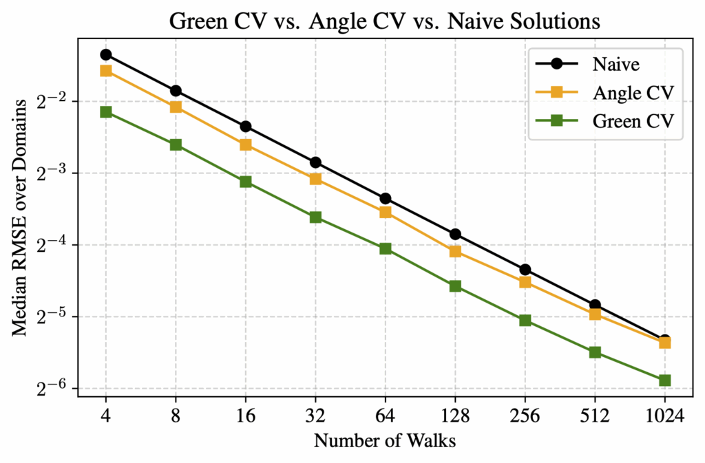
To verify our 2-pass method, we compared it against a reference solution obtained by running WoS with 32,768 walks, which we take as ground truth since this number is sufficient for convergence. For evaluation, we tested using between 4 and 1024 walks, and compared three methods—naive WoS, control variates with the Green’s function, and control variates with the angle kernel. We measured the median RMSE across 20 unique domains relative to the reference solution.
For all experiments, we used the following settings. The grid resolution was \( 256 \times 256 \) and the epsilon shell for WoS was \( 0.001 \). The number of basis functions for the denoiser was \( 80 \) and the number of walks for the samples for the denoisers was \( 128 \). We used \( \ell_2 \) regularization with \( \alpha = 0.1 \). The Dirichlet boundary condition we used is given by:
$$
g(x, y) = \sin\big(5\pi y\big) + \cos\big(2\pi x\big)
$$
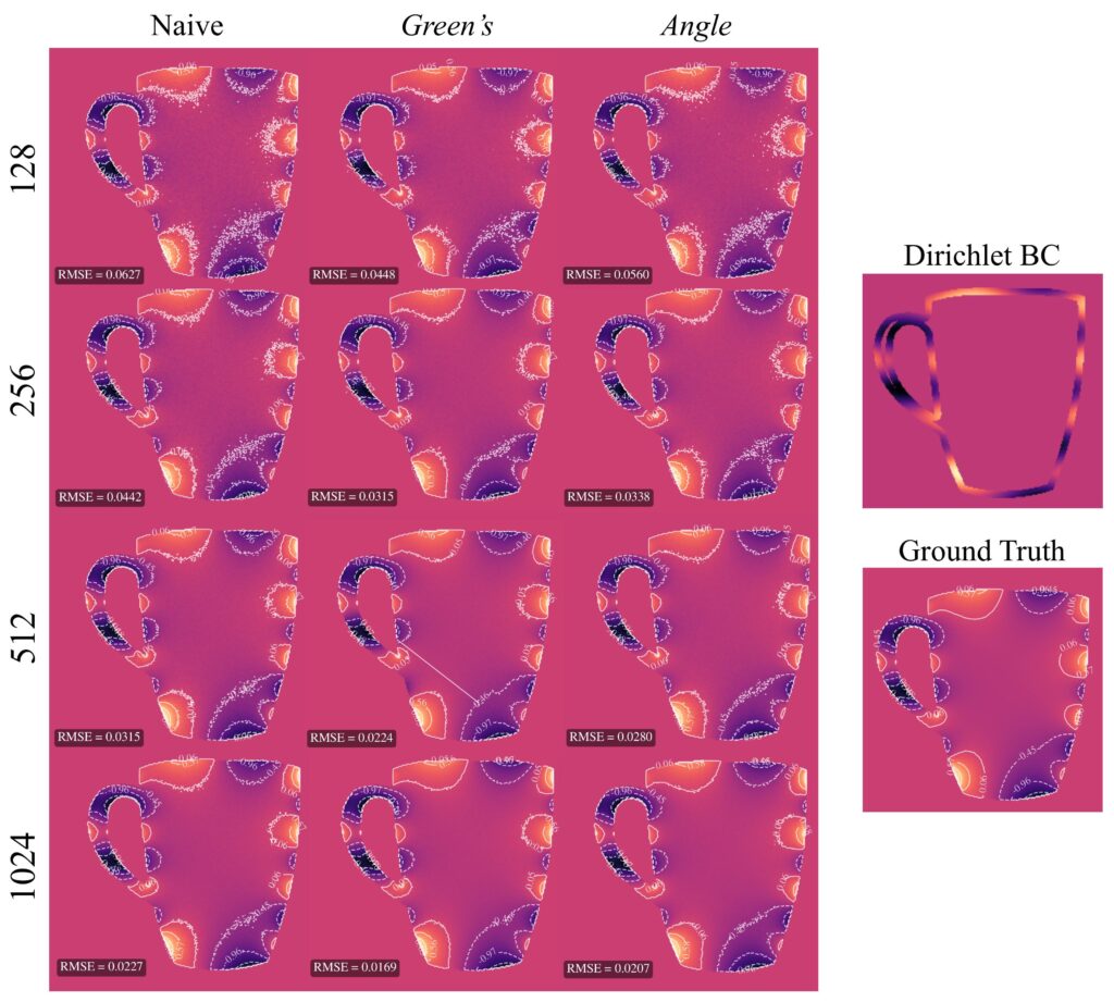
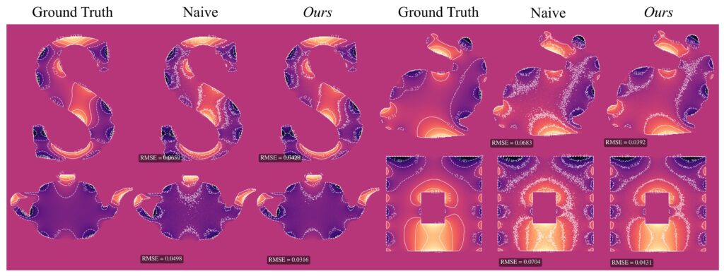
Based on RMSE, we observed that our control variate method for both kernels outperformed the naive WoS on average. The control variate with Green’s theorem showed significant linear improvement as the number of walks increased. The angle kernel did not yield as good results as Green’s; however, in the vast majority of experiments, the angle kernel control variate still achieved better RMSE than naive WoS. The only exception we observed was on more complex domains with a high number of walks. In contrast, for the Green’s kernel, we did not encounter any domain or walk count in which naive WoS outperformed the control variate method.
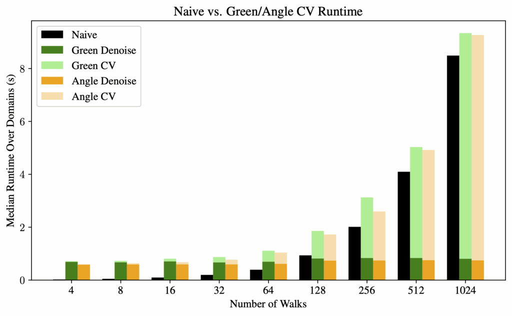
For computation time, we observed that the denoising process has a fixed amount of overhead. Therefore, as the number of walks increases, the denoising time becomes a negligible factor in the overall computation time. The bottleneck is then essentially the same as the naive method: the random walks.
5 Extensions
5. 1 N-Pass Gradient Descent Approach
Building upon the 2-pass harmonic control variate method, we experimented with an n-pass gradient descent approach to iteratively refine the control variate using Monte Carlo estimates as supervision. This method was motivated by the Neural Walk-on-Spheres framework [Nam, Berner, and Anandkumar 2024], which uses a general-purpose neural network \( u_\theta(x) \) as the learned control variate. Our method instead optimizes the coefficient weights \( \sigma ∈ ℝ^{M} \) of a harmonic control variate \( c(x) \), adhering to the structure of the underlying PDE.
The weights \( \sigma \) are initialized from a small set of sample points via the linear system (**), and stochastic gradient descent aims to then minimize the discrepancy between the control variate \( c(x) \) and Monte Carlo estimates \( \langle u(x) \rangle \).
Our optimization loop is implemented as follows:
- Sample a batch of interior points \( x_i \) and compute Monte Carlo estimates \( \langle u(x_i) \rangle \) for each batch point using WoS
- Evaluate the current control variate at each \( x_i \), and compute the mean square error (MSE) loss $$\mathscr{L} = \frac{1}{B} \sum_{i=1}^{B} \left( c(x_i) – \langle u(x_i) \rangle \right)^2$$
- Perform a gradient step on \( \mathscr{L} \) with respect to \( \sigma \) via Adam optimizer
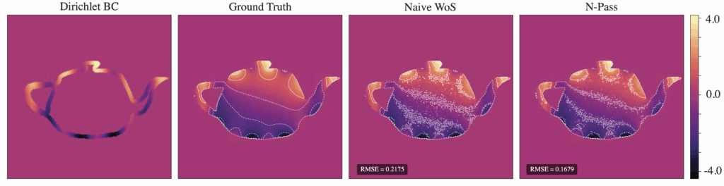
For the same total number of walks, Figure 11 illustrates a significant improvement in RMSE compared to naive WoS, with the contours indicating a much less noisy interpolation of the boundary for our n-pass solution.
Further improvements include accelerating the repeated computation of \( c(x) \), adaptively adjusting the learning rate, and experimenting with different weight initializations. For example, when artifacts appeared in the denoiser due to a large number of monopoles, these artifacts remained present even after the optimization, since weights were initialized based on the denoiser.
5.2 Neumann Boundary Conditions
Many real-world PDE problems involve boundary behavior that is best described by flux, rather than a set of fixed values. Neumann conditions prescribe the normal derivative of the solution along the boundary. In the case of mixed boundary conditions, we seek a function \( u \) satisfying:
$$
\Delta u = 0 \text{ in } \Omega, \quad u = g \text{ on } \partial\Omega_D, \quad \frac{\partial u}{\partial n} = h \text{ on } \partial\Omega_N
$$
where the boundary \( \partial \Omega = \partial \Omega_D \cup \partial\Omega_N \) is partitioned into Dirichlet and Neumann components. A 2-pass approach in this setting would first construct a control variate \( c(x) \approx u(x) \), and estimate the residual \( u(x) – c(x) \) which satisfies:
$$\Delta(u – c) = 0 \text{ in } \Omega, \quad (u – c) = (g – c) \text{ on } \partial\Omega_D, \quad \frac{\partial}{\partial n}(u – c) = h – \frac{\partial c}{\partial n} \text{ on } \partial\Omega_N$$
In particular, when we choose Green’s function for our control variate, the Neumann boundary condition is corrected via the Poisson kernel,
$$\frac{\partial}{\partial n} (u – c)(x) = h(x) – \sum_i \frac{\partial}{\partial n} P(x, y_i) \, \sigma_i,$$
as the Poisson kernel is the normal derivative of the Green’s function with respect to the boundary point:
$$P(x, y) = -\frac{\partial G}{\partial n_y}(x, y), \quad y \in \partial\Omega$$
By using this residual-based formulation, we apply the control variate to both value and flux constraints, enabling variance reduction even in domains with mixed boundaries.
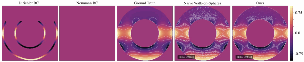
Figure 12. Naive vs. 2-pass method with Dirichlet BC 𝑢 (𝑥, 𝑦) = cos(2𝜋𝑦) and Neumann BC 𝜕𝑢/𝜕𝑛 = 0, num of walks = 128
To handle Neumann boundary conditions, the original WoS algorithm needs to be modified to address the behavior of walks near Neumann boundaries, the radius of closed balls around each point, and conditions for walk termination. The Walk on Stars algorithm (Sawhney et al., 2023) does exactly this. Walk on Stars generalizes WoS by replacing ball-shaped regions with stars — a star being any shape where every boundary point can be “seen” from the centre. At Neumann boundaries, Walk on Stars simulates reflecting Brownian motion — when a walk reaches a Neumann boundary, it is reflected according to the boundary’s normal vector and picks up a contribution of the Neumann condition, \( h \).
Figure 12 illustrates our results with a zero-valued Neumann boundary condition.The 2-pass method still reduces the RMSE compared to Naive WoS with the same number of walks. However, the contours indicate somewhat increased noise near the reflecting boundary compared to the absorbing boundary on our solution.
5.3 Grouping Techniques to Reduce Overfitting and Improve Stability
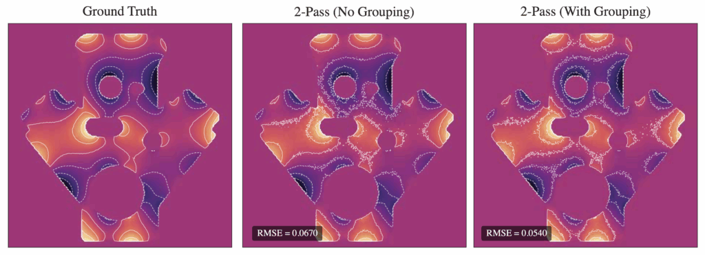
As detailed in Section 3.3, a major consideration when estimating control variates is the conditioning and placement monopoles. To further address this, we experimented with grouping techniques that compress nearby or similar samples and assign them a shared influence, namely:
- Greedy grouping: Choose a point and assign all other points within a fixed radius to one group. Each groups shares either a weight or a single basis function, effectively reducing the number of active degrees of freedom in the system. Our experiments show a reduction in RMSE via grouping for the angle kernel (see Figure 13), but contours indicate a slight increase in noise in some regions.
- DBSCAN: This density-based clustering technique automatically identifies dense clusters of points. Each cluster is treated as a group, and only a representative or averaged contribution is retained, while the rest are collapsed into it.
6 Conclusions and Future Directions
We introduced harmonic control variates: a simple, closed-form control variate for Walk-on-Spheres built from mixtures of harmonic kernels. By fitting a lightweight least-squares model once and efficiently evaluating it in closed form during sampling, we turn WoS into a two-pass estimator that remains unbiased while substantially lowering variance. Empirically, our method delivers consistent accuracy gains across diverse geometries—e.g., an average 40% RMSE reduction at 128 walks—while adding only minimal overhead compared to previous neural control variate approaches; as walks dominate runtime, the extra cost is effectively negligible. The result is a method that is easy to implement (a small change to a standard WoS pipeline), robust to geometric complexity, and markedly more sample-efficient.
Future work. We plan to release a plug-in that drops into existing WoS codebases and to continue improving our method for even stronger variance reduction at essentially the same runtime.
References
Jacobson, Alec, Ladislav Kavan, and Olga Sorkine [2013]. “Robust Inside-Outside Segmentation using Generalized Winding Numbers”. In: ACM Trans. Graph. 32.4.
Li, Zilu et al. [2024]. “Neural Control Variates with Automatic Integration”. In: ACM SIGGRAPH 2024 Conference Papers. SIGGRAPH ’24. Denver, CO, USA: Association for Computing Machinery. isbn: 9798400705250. doi: 10.1145/3641519. 3657395. url: https://doi.org/10.1145/3641519.3657395.
Madan, Abhishek et al. [July 2025]. “Stochastic Barnes-Hut Approximation for Fast Summation on the GPU”. In: Proceedings of the Special Interest Group on Computer Graphics and Interactive Techniques Conference Conference Papers. SIGGRAPH Conference Papers ’25. ACM, pp. 1–10. doi: 10.1145/3721238.3730725. url: http://dx.doi.org/10.1145/3721238.3730725.
Muller, Mervin E. [1956]. “Some Continuous Monte Carlo Methods for the Dirichlet Problem”. In: The Annals of Mathematical Statistics 27.3, pp. 569–589. doi: 10.1214/aoms/1177728169. Url: https://doi.org/10.1214/aoms/1177728169.
Nam, Hong Chul, Julius Berner, and Anima Anandkumar [2024]. “Solving Poisson Equations Using Neural Walk-on-Spheres”. In: Forty-first International Conference on Machine Learning
Sawhney, Rohan and Keenan Crane [Aug. 2020]. “Monte Carlo geometry processing: a grid-free approach to PDE-based methods on volumetric domains”. In: ACM Trans. Graph. 39.4. issn: 0730-0301. Doi: 10.1145/3386569.3392374. url: https://doi.org/10.1145/3386569.3392374.
Sawhney, Rohan and Bailey Miller [2023]. Zombie: Grid-Free Monte Carlo Solvers for Partial Differential Equations. Version 1.0.
Sawhney, Rohan, Bailey Miller, et al. [July 2023]. “Walk on Stars: A Grid-Free Monte Carlo Method for PDEs with Neumann Boundary Conditions”. In: ACM Trans. Graph. 42.4. issn: 0730-0301. doi: 10.1145/3592398. url: https://doi.org/10.1145/3592398.