An Open Challenge
The goal of this post is to celebrate the question. History’s greatest intellectual leaps often began not with the answer itself, but with the journey of tackling a problem. Hilbert’s 23 problems charted the course of a good chunk of 20th-century mathematics. Erdős scattered challenges that lead to breakthroughs in entire fields. The Millennium Prize Problems continue to inspire and frustrate problem solvers.
There’s magic in a well-posed problem; it ignites curiosity and forces innovation. Since I am nowhere near the level of Erdős or Hilbert, today, we embrace that spirit with a maybe less well-posed but deceptively simple yet intriguing geometric puzzle on a disordered surface.
To this end, we present a somewhat geometric-combinatorial problem that bridges aspects of computational geometry, bond percolation theory and graph theory.
Problem Construction
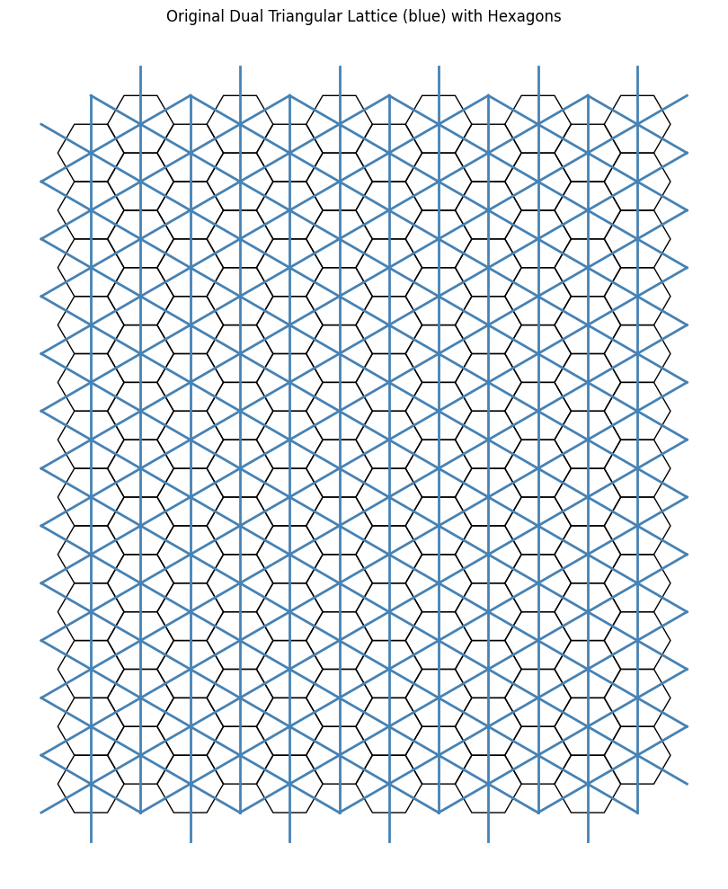
We begin with the hexagonal lattice in \(\mathbb{R}^2\) (the two-dimensional plane), specifically the regular hexagonal lattice (also known as the honeycomb lattice). For visualisation, a finite subregion of this lattice tessellation of the plane is illustrated below.
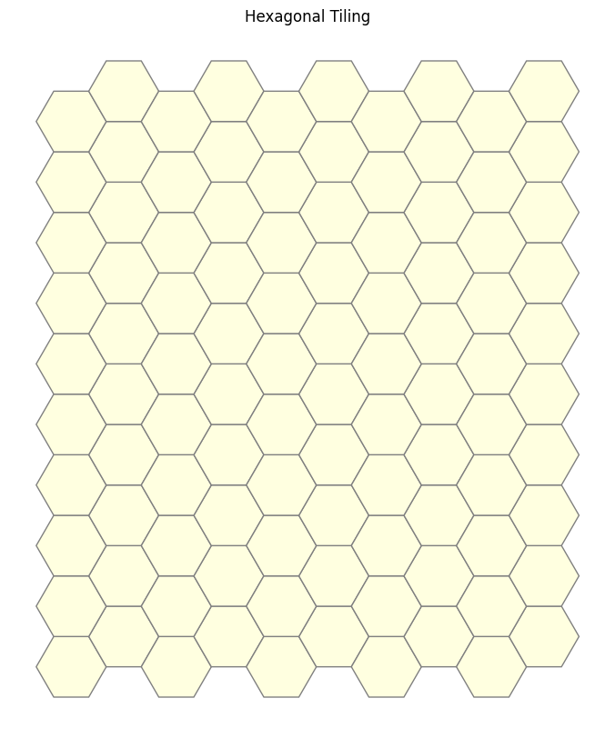
We then enrich the information of our space by constructing centroids associated with each hexagon in the lattice. The guiding idea is to represent each face of the lattice by its centroid, treating these points as abstract proxies for the faces themselves.
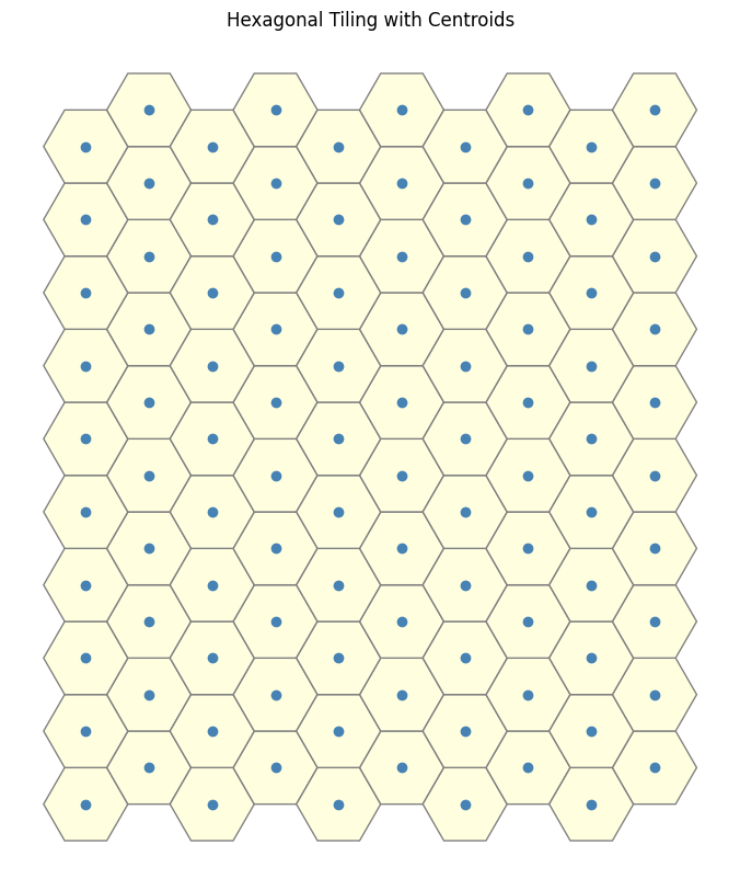
These centroids are connected precisely when their corresponding hexagons share a common edge in the original lattice. Due to the hexagonal tiling’s geometry, this adjacency pattern induces a regular network of connections between centroids, reflecting the staggered arrangement of the hexagons.
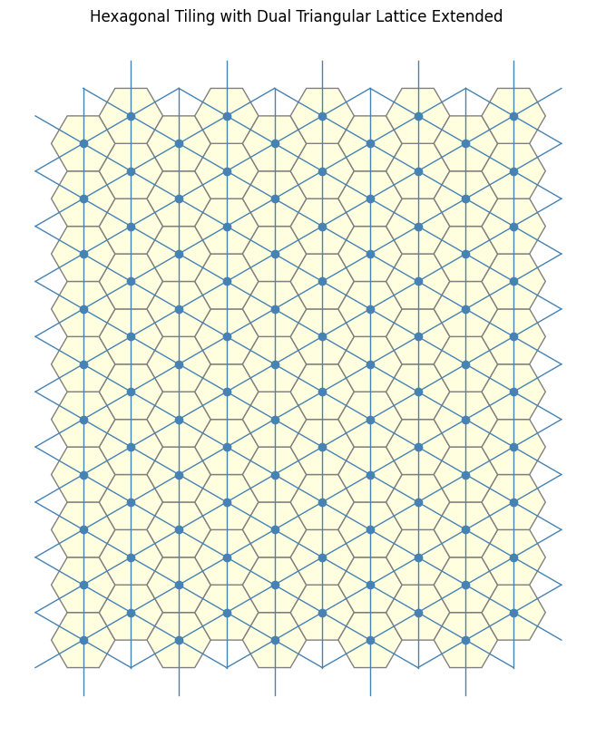
This process yields a new structure: the dual lattice. In this case, the resulting dual is the triangular lattice.This dual lattice encodes the connectivity of the original tiling’s faces through its vertices and edges.
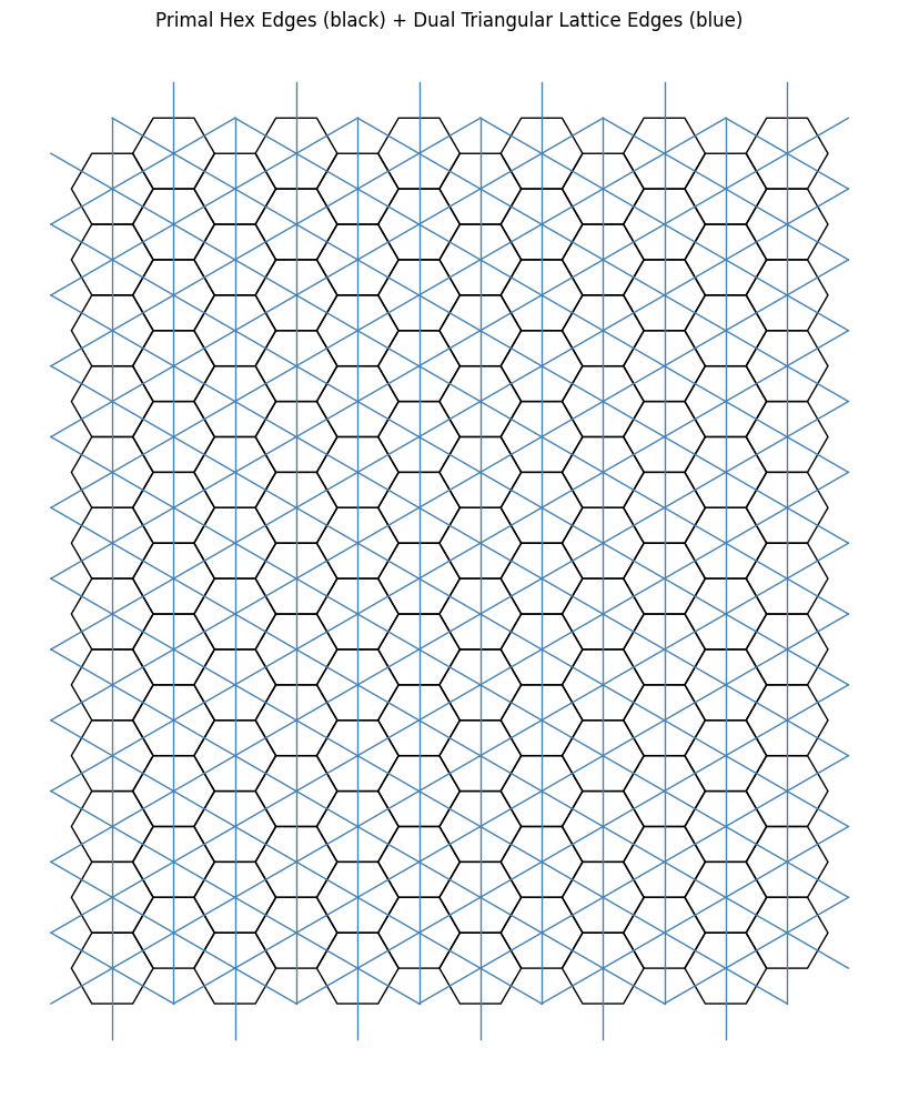
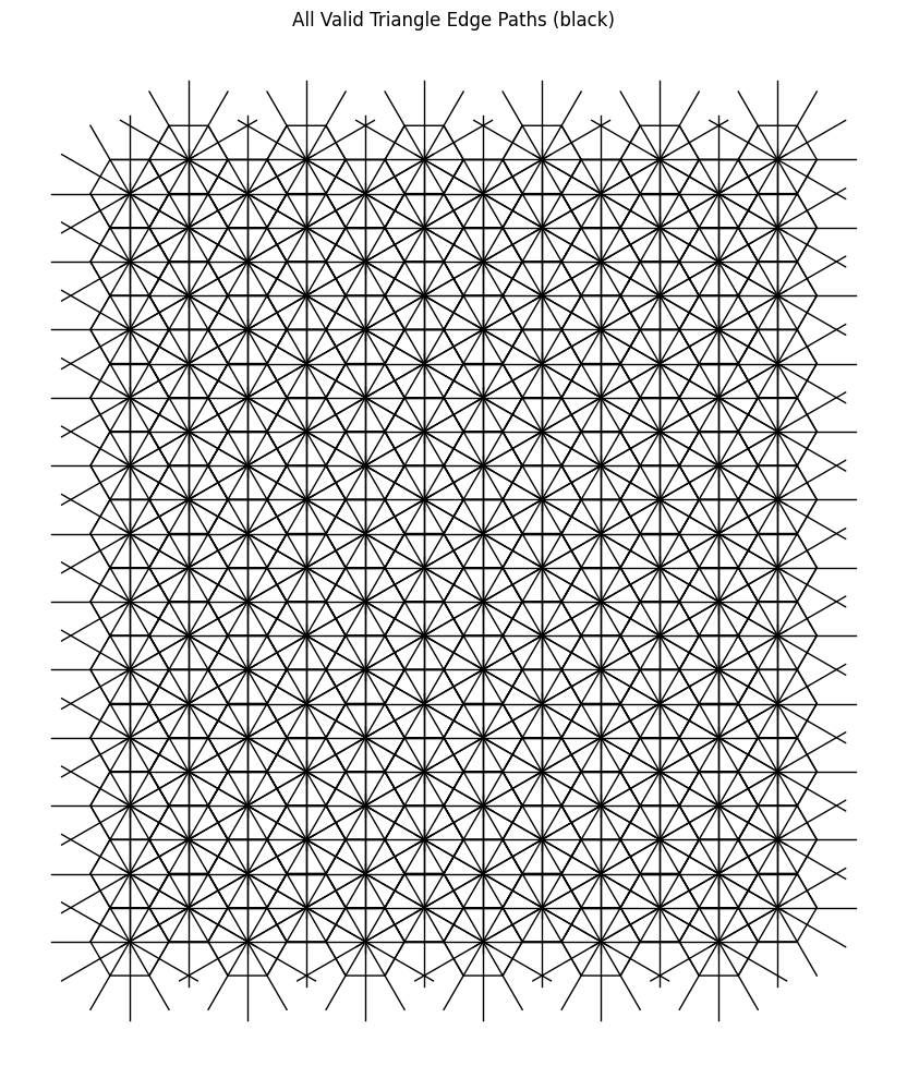
As a brief preview of the questions to come, our goal is to identify triangles within this expansive lattice. We begin by requiring that the vertices of these triangles originate from the centroids of the hexagonal faces. To then encode such triangular structures, we leverage both the primal and dual lattices, combining them so that the edges of these triangles can exist on any of the black paths shown in the diagram.
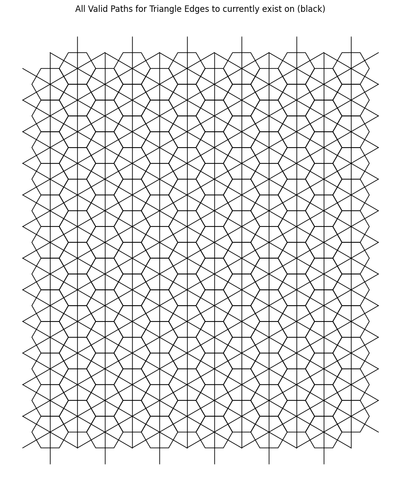
What is particularly interesting here is that the current construction arises from 1-neighbor connections, which we interpret as close-range interactions. However, this 1-neighbor primal-dual framework restricts the set of possible triangles to only equilateral ones. (Personally, I feel this limits the complexity of potential problems.)
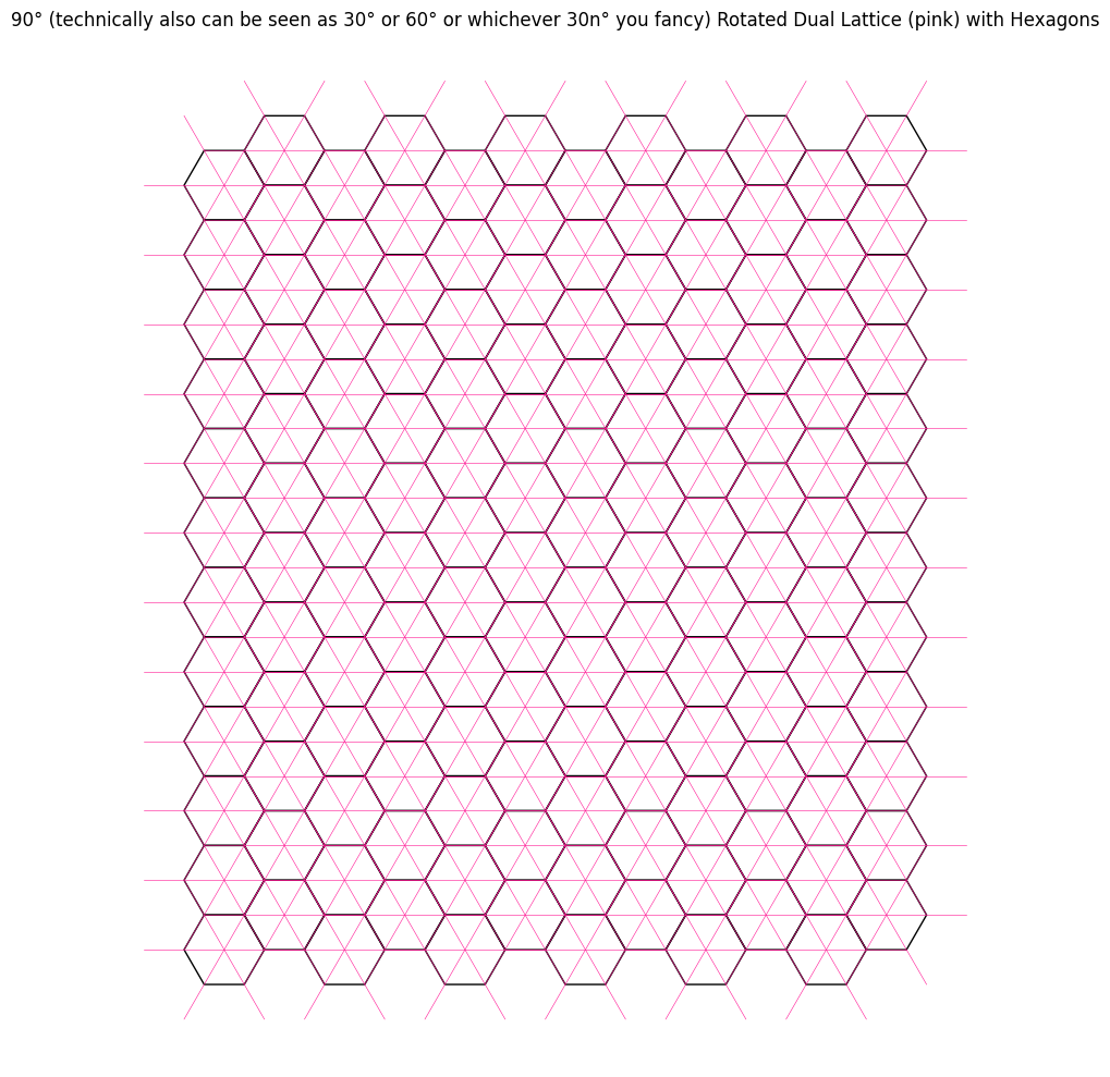
To make the question more engaging and challenging, we seek to incorporate more “medium-to-further-range interactions“. This can be accomplished by connecting every second neighbor in an analogous fashion, thereby constructing a “triple space“. The resulting structure forms another dual lattice that captures these extended adjacency relations, allowing for a richer variety of triangular configurations beyond the equilateral case. For generality, I will coin the term for this as 2-close-range-interactions.
A lazy yet elegant approach to achieve this is by rotating the original dual lattice by \(90\) degrees, or, more generally, by any multiple of \(30\) degrees (i.e., \(30 \times n\) degrees , we will use this generality in the final section to extend the problem scope even further). We then combine this rotated lattice with the original construction.
We will illustrate the process below.
The 2-close-range interaction:
We begin, as before, with the original primal and dual lattices.
We now rotate the blue dual lattice by \(90\) degrees, as described previously.
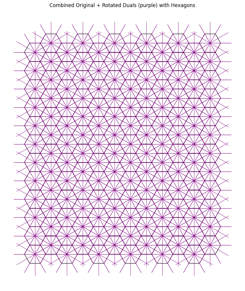
Combining the rotated dual with the original, as before, yields the following structure and, as the keen eyed among you may notice, both the dual constructions covers the entire original primal hexagonal lattice.
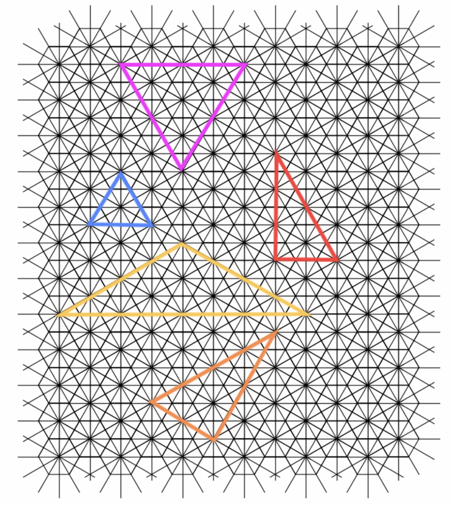
This finally yields us the following existence space for the triangles.
And now, we witness the emergence of a richer and more interesting variety of triangle configurations.
The Random Interface
To introduce an interesting stochastic element to our problem, we draw inspiration from percolation theory (a framework in statistical physics that examines how randomness influences the formation of connected clusters within a network). Specifically, we focus on the concept of disorder, exploring how the presence of randomness or irregularities in a system affects the formation of connected clusters. In our context, this translates to the formation of triangles within the lattice.
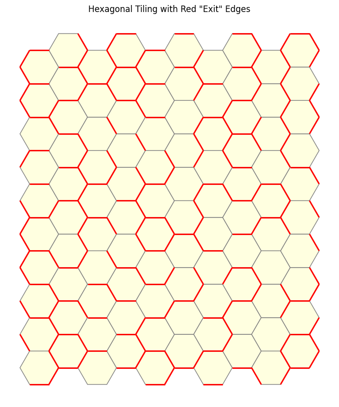
Building upon the original hexagonal lattice, we assign to each edge a probability \(p\) of being “open” or “existent”, and consequently, a probability \(1 – p\) of being “closed” or “nonexistent”. This approach mirrors the bond percolation model, where edges are randomly assigned to be open or closed, independent of other edges. The open edges allow for the traversal of triangle edges, akin to movement through a porous medium, facilitating the formation of triangles only through the connected open paths.
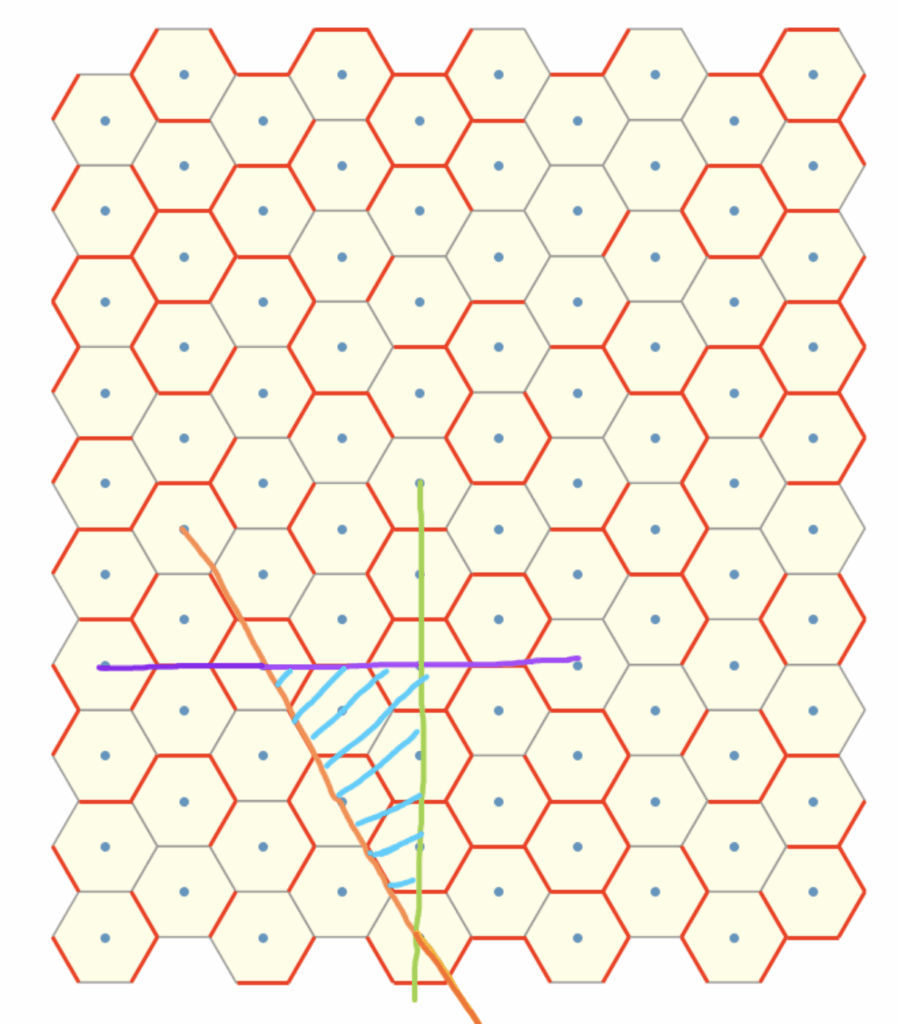
We illustrate using the figure a sample configuration when \(p = 0.5\), where the red “exit” edges represent “open” edges that allow triangles to traverse through the medium.
Rules regarding traversal of this random interface:
As mentioned earlier, every red “open” gate permits traversal. To define this traversal more clearly in our problem setting, we can visualise using the following.
In the 2-close-range interaction case, this traversal is either in the tangential direction
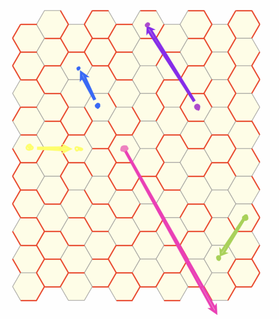
or in the normal direction.
An aside on Interaction Modeling
This model assumes that long-range interactions emerge from specified short-range interactions. We can see this in our construction of the 2-close explicitly excluding any secondary dual lattice edges (2-close interactions) that can be generated from first-neighbor edges (1-close interactions). This ensures that the secondary dual lattice contains only truly second-neighbor interactions not implied by (or that goes through) the first-neighbor structure, preserving a clear hierarchical interaction scheme.
The Problems
An “Easy” starting question :
Given some finite subsection of this random interface, construct an algorithm to find the largest triangle (in terms of perimeter or area, your choice of definition for the problem depending on which variant of the problem you want to solve) .
Attempt at formalising this
1) Definition of Lattices
Hexagon Lattice
Let the hexagonal lattice be denoted by:
$$
H = (C, E_h)
$$
where:
- \(C = { c_i } \subset \mathbb{R}^2\) is the set of convex hexagonal cells that partition the Euclidean plane \(\mathbb{R}^2\),
- \(E_h = { (c_i, c_j) \in C \times C \mid c_i \text{ and } c_j \text{ share a common edge} }\) is the adjacency relation between hexagons.
Each hexagon edge \(e_h \in E_h\) is activated independently with probability \(p \in [0,1]\):
$$
\Pr(\sigma_h(e_h) = 1) = p, \quad \Pr(\sigma_h(e_h) = 0) = 1-p
$$
Primary Dual Lattice \(T_1 = (V, E_t^{(1)})\)
The primary dual lattice connects centroids of adjacent hexagons:
$$
E_t^{(1)} = \left \{ (v_i, v_j) \in V \times V \,\middle|\, (c_i, c_j) \in E_h \right \}
$$
Secondary Dual Lattice \(T_2 = (V, E_t^{(2)})\)
The secondary dual lattice captures 2-close interactions. An edge \((v_i, v_j) \in E_t^{(2)}\) exists if and only if:
- \(c_i \neq c_j\) and \((v_i, v_j) \notin E_t^{(1)}\) (i.e., not first neighbors),
- There exists a common neighboring cell \(c_k \in C\) such that:
$$
(c_i, c_k) \in E_h \quad \text{and} \quad (c_j, c_k) \in E_h
$$ - The straight-line segment \(\overline{v_i v_j}\) does not lie entirely within \(c_i \cup c_j \cup c_k\):
$$
\overline{v_i v_j} \not\subseteq c_i \cup c_j \cup c_k
$$
Hence, the formal definition:
$$
E_t^{(2)} = \left\{ (v_i, v_j) \in V \times V \ \middle| \
\begin{aligned}
& c_i \ne c_j,\ (v_i, v_j) \notin E_t^{(1)}, \
& \exists\, c_k \in C:\ (c_i, c_k), (c_j, c_k) \in E_h, \
& \overline{v_i v_j} \not\subseteq c_i \cup c_j \cup c_k
\end{aligned}
\right\}
$$
Combined Dual Lattice
The complete dual lattice is defined as:
$$
T = (V, E_t), \quad \text{where} \quad E_t = E_t^{(1)} \cup E_t^{(2)}
$$
2) Edge Activation
Hexagon Edge Activation
Each hexagon edge \(e_h \in E_h\) is independently activated with probability \(p\) as:
$$
\sigma_h(e_h) \sim \text{Bernoulli}(p)
$$
Dual Edge Activation
Each dual edge \(e = (v_i, v_j) \in E_t\) has an activation state \(\sigma(e) \in \{0,1\}\) defined by the following condition:
$$\sigma(e) = 1 \quad \text{if } \overline{v_i v_j} = or \perp e_h \in E_h \text{ and } \sigma_h(e_h) = 1;
\
\sigma(e) = 0 \quad \text{otherwise}$$
In other words, a dual edge is activated only if it corresponds spatially to a hexagon edge that is itself activated, either by lying exactly on it or intersecting it at right angles.
3) Interaction Constraints
Local Traversal: Paths across the lattice are constrained to activated edges:
$$
P(v_a \rightarrow v_b) = { e_1, e_2, \dots, e_k \mid \sigma(e_i) = 1,\ e_i \in E_t }
$$
Cardinality:
$$
\deg_{T_1}(v_i) \leq 6, \quad \deg_{T_2}(v_i) \leq 6
$$
Each vertex connects to at most 6 first neighbors (in \(T_1\)) and at most 6 geometrically valid second neighbors (in \(T_2\)).
4) Triangle Definition
A valid triangle \(\Delta_{abc} = (v_a, v_b, v_c)\) must satisfy:
- Connectivity: All three edges are activated:
$$
\sigma(v_a v_b) = \sigma(v_b v_c) = \sigma(v_c v_a) = 1
$$ - Embedding: The vertices \((v_a, v_b, v_c)\) form a non-degenerate triangle in \(\mathbb{R}^2\), preserving local lattice geometry.
- Perimeter: Defined as the total edge length:
$$
P(\Delta_{abc}) = |v_a – v_b| + |v_b – v_c| + |v_c – v_a|
$$ - Area: Using the standard formula for triangle area from vertices:
$$
A(\Delta_{abc}) = \frac{1}{2} \left| (v_b – v_a) \times (v_c – v_a) \right|
$$
where \(\times\) denotes the 2D scalar cross product (i.e., determinant).
Triangles may include edges from either \(E_t^{(1)}\) or \(E_t^{(2)}\) as long as they meet the activation condition.
5) Optimization Objective
Given the dual lattice \(T = (V, E_t)\) and activation function \(\sigma: E_t \rightarrow \{0,1\}\), the goal is to find the valid triangle maximizing either:
- Perimeter:
$$
\underset{\Delta_{abc}}{\mathrm{argmax}} \; P(\Delta_{abc})
$$ - Area:
$$
\underset{\Delta_{abc}}{\mathrm{argmax}} \; A(\Delta_{abc})
$$
subject to \(\Delta_{abc}\) being a valid triangle.
Harder Open Questions:
1) What are the scaling limit behaviors of the triangle structures that emerge as the lattice size grows?
In other words: As we consider larger and larger domains, does the global geometry of triangle configurations converge to some limiting structure or distribution?
Ideas to explore:
Do typical triangle shapes concentrate around certain forms?
Are there limiting ratios of triangle types (e.g., equilateral vs. non-equilateral)?
Does a macroscopic geometric object emerge (in the spirit of scaling limits in percolation, e.g., SLE curves on critical lattices)?
An attempt to formalise this would be as follows :
Let’s denote by \(T_p(L)\) the set of all triangles that can be formed inside a finite region of side length \(L\) on our probabilistic lattice, where each edge exists independently with probability \(p\).
Conjecture: As \(L\) becomes very large (tends to infinity), the distribution of triangle types (e.g. equilateral, isosceles, scalene, acute, obtuse, right-angled) converges to a well-defined limiting distribution that depends only on \(p\). (i.e converges in law to some limiting distribution \(\mu_p\). )
Interpretation of expected behaviours:
- For high \(p\) (near 1), most triangles are close to equilateral.
- For low \(p\) (near 0), triangles become rare or highly irregular.
- This limiting distribution, \(\mu_p\) , tells us the “global shape profile” of triangles formed under randomness.
2) How does the distribution of triangle types (e.g., equilateral, isosceles, scalene; or acute, right, obtuse) vary with the probability parameter \(p\)?
Why this matters: At low \(p\), triangle formation is rare, and any triangle that does form may be highly irregular. As \(p\) increases, more symmetric (or complete) structures may become common.
Possible observations:
Are equilateral triangles more likely to survive at higher \(p\) due to more consistent connectivity?
Do scalene or right-angled triangles dominate at intermediate values of \(p\) due to partial disorder?
Is there a characteristic “signature” of triangle types at criticality?
3) Can we define an interesting phase transition in this setting, marking a shift in the global geometry of the triangle space?
In other words: As we gradually increase the edge probability $p$, at what point does the typical shape of the triangles we find change sharply?
An attempt to formalise this would be as follows :
There exist two critical probability values \(p_1\) and \(p_2\) (where \(0 < p_1 < p_2 < 1\)) that mark qualitative transitions in the kinds of triangles we typically observe.
Conjecture:
- When \(p < p_1\), most triangles that do form are highly irregular (i.e scalene).
- When \(p_1 < p < p_2\), the system exhibits a diverse mix of triangle types (now we have more equilateral, isosceles with less domination of scalene; and variations of acute, right-angled, and obtuse).
- When \(p > p_2\), the triangles become increasingly regular, and equilateral triangles dominate.
This suggests a “geometric phase transition” in the distribution of triangle shapes, driven purely by the underlying connectivity probability.
4) Is there a percolation threshold at which large-scale triangle connectivity suddenly emerges?
Let’s define a triangle cluster as a set of triangles that are connected via shared edges or vertices (depending on your construction). We’re interested in whether such triangle clusters can become macroscopically large.
Conjecture:
There exists a critical probability \(p_c\) such that:
- If \(p < p_c\), then all triangle clusters are finite (they don’t span the system).
- If \(p > p_c\), then with high probability (as the system size grows), a giant triangle cluster emerges that spans the entire domain.
This is analogous to the standard percolation transition, but now with triangles instead of edge or site clusters.
(The first attempt setting up this was whether a single giant triangle can engulf the whole space but in retrospect, this would not be possible and is not such an interesting question.)
5) Results on Triangle Density
As we grow the system larger and larger, does the number of triangles per unit area settles down to a predictable average, but this average depends heavily on the edge probability $p$.
Let \(N_p(L)\) denote the total number of triangles formed within a square region of side length \(L\).
We define the triangle density as
$$
\rho_p(L) := \frac{N_p(L)}{L^2},
$$
which is the average number of triangles per unit area.
Conjecture: As \(L \to \infty\), the triangle density converges to a deterministic function \(\rho(p)\):
$$
\lim_{L \to \infty} \rho_p(L) = \rho(p).
$$
(Here, \(\rho(p)\) captures the asymptotic average density of triangles in the infinite lattice for edge probability \(p\).)
Furthermore, the variance of \(N_p(L)\) satisfies
$$
\mathrm{Var}[N_p(L)] = o(L^4),
$$
(i.e variance of the number of triangles grows more slowly than the square of the area)
which implies the relative fluctuations:
$$
\frac{\sqrt{\mathrm{Var}[N_p(L)]}}{L^2} \to 0.
$$
vanish as \(L \to \infty\).
The function \(\rho(p)\) is analogous to the percolation density in classical bond percolation, which measures the expected density of occupied edges or clusters. Just as percolation theory studies the emergence and scaling of connected clusters, here \(\rho(p)\) characterizes the density of geometric structures (triangles) emerging from random edge configurations.
The sublinear variance scaling reflects a law of large numbers effect in spatial random graphs: as the region grows, the relative randomness in triangle counts smooths out, enabling well-defined macroscopic statistics.
This parallels known results in random geometric graphs and continuum percolation, where densities of subgraph motifs stabilize in large limits. This behavior may also hint at connections to scaling exponents or universality classes from statistical physics. (With certain constraints, could classify the triangles or regions of connected triangles as interfaces and make connections with KPZ type problems too, possibly another conjecture but I think 5 problems to think about are more than enough for now.)
What are some applications?
While I approach this problem primarily from a theoretical lens, with an interest in its mathematical structure and the questions it naturally raises, I also recognize that others may find motivation in more tangible or applied outcomes. To speak to that perspective, I include two detailed examples that illustrate how ideas from this setting can extend into meaningful real-world contexts. The aim is not to restrict the problem’s scope to practical ends, but to show how the underlying tools and insights may resonate across domains and disciplines.
—–//—–
Application 1
1) Retopology of a 3D Scan
Consider the setting of high-resolution 3D scanning, where millions of sample points capture the geometry of a complex surface. These points are typically distributed (or essentially clumped) within an \(\varepsilon\)-thick shell around the true surface geometry, often due to the scan exhibiting local noise, redundancy, or sampling irregularities. Within this context, our framework finds a natural interpretation.
One can view the scan as a point cloud embedded on a virtual, warped hexagonal lattice, where the underlying lattice geometry adapts to local sampling density. By introducing a probability field, governed by factors such as local curvature, scan confidence, or spatial regularity, we assign likelihoods to potential connections between neighboring points.
In this formulation, the task of finding large, connected configurations of triangles corresponds to the process of identifying coherent, semantically meaningful patches of the surface. These patches serve as candidates for retopologization (the construction of a low-resolution, structured mesh that preserves the essential geometric features of the scan while filtering out noise and redundancies). This resulting mesh is significantly more amenable to downstream applications such as animation, simulation, or interactive editing.
The nearest-neighbor locality constraint we impose reflects a real physical prior, i.e mesh edges should not “jump” across unconnected regions of the surface. This constraint promotes local continuity and geometric surface fidelity.
Application 2
2) Fault Line Prediction in Material Fracture
In materials science, understanding how fractures initiate and propagate through heterogeneous media is a central problem. At microscopic scales, materials often have grain boundaries, impurities, or irregular internal structures that influence where and how cracks form. This environment can be abstracted as a disordered graph or lattice, where connections (or lack thereof) between elements model structural integrity or weakness.
We can reinterpret such a material as a random geometric graph laid over a deformed hexagonal lattice, with each connection representing a potential atomic or molecular bond. Assign a probability field to each edge, governed by local stress, strain, or material heterogeneity, capturing the likelihood that a bond remains intact under tension.
Triangles in this setting can be thought of as minimal stable configurations. As stress increases or defects accumulate, connected triangle structures begin to break down. By tracking the largest connected triangle regions, one may identify zones of high local integrity, while their complement reveals emergent fault lines, regions where fracture is likely to nucleate.
Thus, searching for maximal triangle clusters under stochastic constraints becomes a method for predicting failure zones before actual crack propagation occurs. Moreover, one can study how the geometry and size distribution of these triangle clusters vary with external stress or material disorder, giving rise to scaling laws or percolation-like transitions.
This formulation connects naturally with known models of fracture networks, but adds a new geometric lens: triangulated regions become proxies for mechanical stability, and their disintegration offers a pathway to understand crack emergence.
—–//—–
Again these are just two specific lenses. At its core, the problem, finding large-scale, connected substructures under local stochastic constraints, arises across many domains. It is easy to reformulate and adjust the constraints to use the tools developed here in other problems.
Auxiliary Insights
When constructing triangles, one can consider the set of paths accessible from a single vertex. To aid visualization, refer to the diagram below.
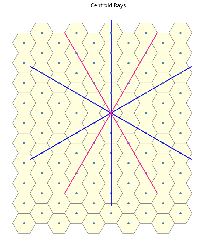
The blue paths are from the 1-close connections, while the pink paths correspond to 2-close connections. Together, they provide each vertex with a total of \(6 + 6 = 12\) possible directions or “degrees of freedom” along which it may propagate to form triangle edges.
Notably, the system exhibits a high degree of rotational symmetry, both the 1-close and 2-close path structures are invariant under rotations by \(60^\circ\). This symmetry can potentially be leveraged to design efficient search algorithms or classification schemes for triangle types within the lattice.
Extension to the n-close case
So far, we’ve been using triangles as a proxy for a special class of simple closed-loop interaction pathways (i.e structures formed by chaining together local movements across the lattice). Specifically we restricted ourselves to the 1- and 2-close interaction setting.
Naturally, a question arises: can we generalize this further? Specifically, what sort of angular adjustment or geometric rule would be needed to define an n-close interaction, beyond the 1- and 2-close cases we’ve explored? (When looking above at the auxillery and the construction of the 2-close, we can see that we use the \(30\) degree rotation offset at the basis.)
This leads to a broader and richer family of questions. In my other blog post (will be linked soon after it is posted) , I’ll pose precisely this: “How can we extend the 2-close interaction to a general n-close interaction?” . There, I’ll also provide a closed-form formula for generating any term in the sequence of such $n$-close interactions.
As always, I encourage you to attempt the question yourself before reading the solution, it may seem straightforward at first, but the correct sequence or geometric structure is not always immediately obvious.
Final Thoughts
Crafting this problem, presenting some drawings and formalising certain aspects was an interesting challenge for me. As always, I welcome any feedback on how to improve the presentation or to formalise certain sections more rigorously if you have any ideas. I’m especially looking forward to seeing and reading about any progress made on the questions posed here, attempts at their variations, or even presentation of potential applications.
Cheers and have an hex-traordinary day ahead!
Srivathsan Amruth
i.e The writer of thismasterpiecechaotic word salad, who apologizes for your lost minutes
Hey, why are you still reading? … Shouldn’t you be pretending to work? ; – )