Intro
Now that you’ve gotten the grasp of meshes, and created your very first 3D object on Polyscope, what can we do next? On Day 4 of the SGI Tutorial Week, we had speakers Richard Liu and Dale Decatur from the Threedle Lab at UChicago explaining about Texture Optimization.
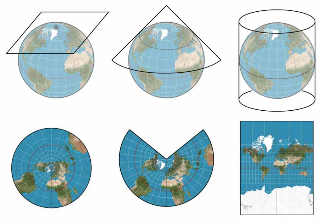
In animated movies and video games, we are used to observing them with realistic textures. Intuitively, we might imagine that we have this texture as a map applied as a flat “sticker” over it. However, we know from some well-known examples in cartography that it is difficult to create a 2D map of a 3D shape like the Earth without introducing distortions or cuts.
Besides, ideally, we would want to be able to transition from the 2D to the 3D map interchangeably. Framing this 2D map as a function on \(\mathbb{R^2}\), we would like it to be bijective.
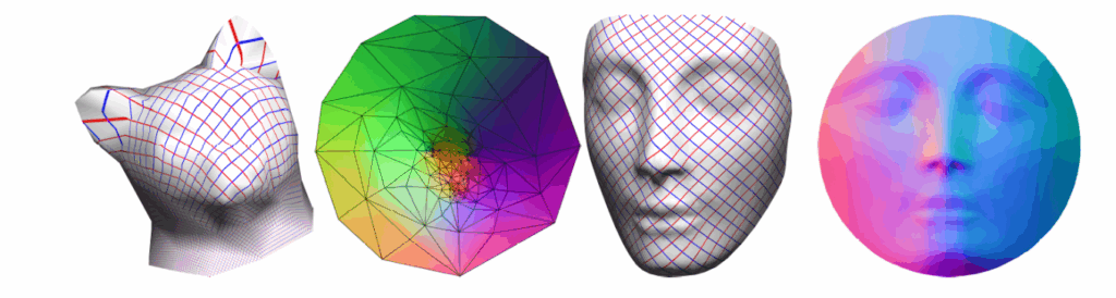
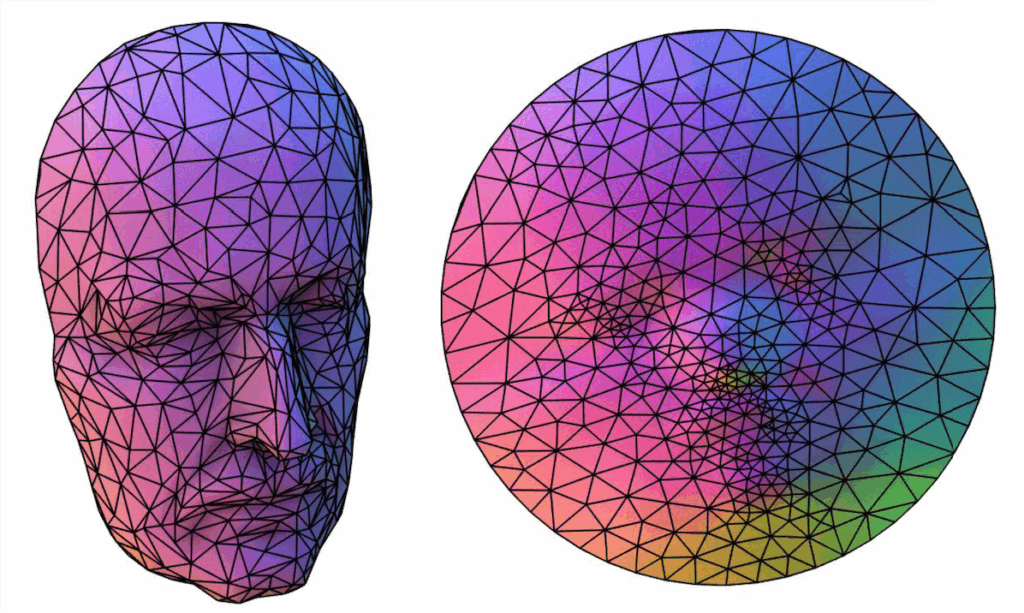
The process of creating a bijective map from a mesh S in \(\mathbb{R^3}\) to a given domain \(\Omega\), or \(F: \Omega \leftrightarrow S\), is known as mesh parametrization.
UV Unwrapping
Consider a mesh defined by the object as \(M = {V, E, F}\), with Vertices, Edges and Faces respectively, where:
\begin{equation*} V \subset R^3 \end{equation*} \begin{align*} E = \{(i, j) \quad &| \text{\quad vertex i is connected to vertex j}\} \\ F = \{(i, j, k) \quad &| \quad \text{vertex i, j , k share a face}\} \end{align*}For a mesh M, we define the parametrization as a function mapping vertices \(V\) to some domain \(\Omega\)
\begin{equation*} U: V \subset \mathbb{R}^3 \rightarrow \Omega \subset \mathbb{R}^2 \end{equation*}For every vertex \(v_i\) we assign a 2D coordinate \(U(v_i) = (u_i, v_i)\) (this is why the method is called UV unwrapping).
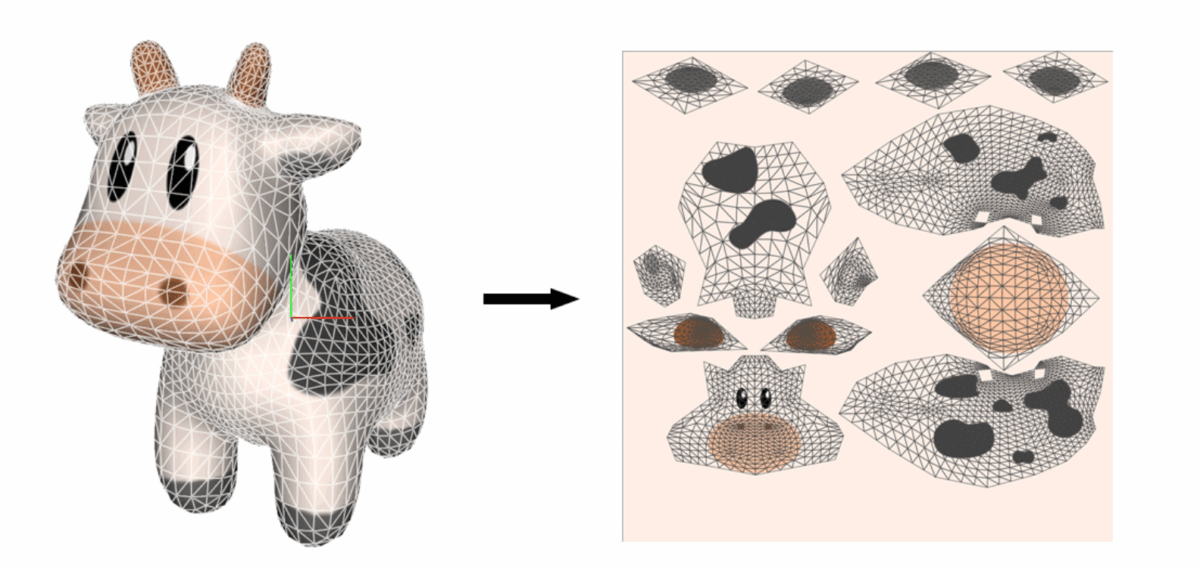
This parametrization has a constraint, however. Only disk topology surfaces (those with a 1 boundary loop) surfaces admit a homeomorphism (a continuous and bijective map) to the bounded 2D plane.
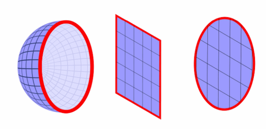
As a workaround, we can always introduce a cut.
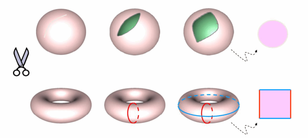
However, these seams create discontinuities, and in turn, distortions we want to minimize. We can distinguish different kinds of distortions using the Jacobian, the matrix of all first-order partial derivatives of a vector-valued function. Specifically, we look at the singular values of the Jacobian (which in the UV function is defined as a 2×3 matrix per triangle).
\begin{align*} J_f = U\Sigma V^T = U \begin{pmatrix} \sigma_1 & 0 \\ 0 & \sigma_2 \\ 0 & 0 \end{pmatrix} V^T \\ f \text{ is equiareal or area preserving} \Leftrightarrow \sigma_1 \sigma_2 &= 1 \\ f \text{ is equiareal or area preserving} \Leftrightarrow \sigma_1 &= \sigma_2 \\ f \text{ is equiareal or area preserving} \Leftrightarrow \sigma_1 &= \sigma_2 = 1 \end{align*}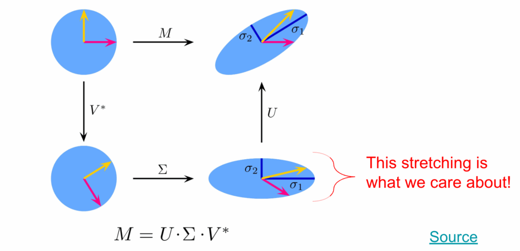
We can find the Jacobians of the UV map assignment \(U\) using the mesh gradient operator \(G \in \mathbb{R}^{3|F|\times V}\)
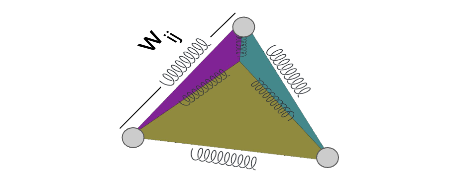
\begin{align*} GU = J \in \mathbb{R}^{3|F|\times V} \end{align*}The classical approach for optimizing a mesh parametrization is viewing the mesh surface as the graph of a mass-spring system (least squares optimization problem). The mesh vertices are the nodes (with equal mass) with each edge acting as a spring with some stiffness constant.
Two key design choices in setting up this problem are:
- Where to put the boundary?
- How to set the spring weights (stiffness)?
To compute the parametrization, we minimize the sum of spring potential energies.
\begin{align*} \min_U \sum_{\{i, j\} \in E} w_ij || u_i – u_j||^2 \end{align*}Where \(u_i = (u_i, v_i)\) is the UV coordinate to vertex i. We then aim to solve the ODE:
\begin{align*} \frac{\partial E}{\partial u _i }= \sum_{j \in N_i} 2 \cdot w_{ij} (u_i – u_j) = 0 \end{align*}Where \(N_i\) indexes all neighbors of vertex \(i\). We can now fix the boundary vertices and solve each equation for the remaining \(u_i\).
A solution by Tutte (1963) and Floater (1997) was computed such that if the boundary is convex and the weights are positive, the solution is guaranteed to be injective. While an injective map has its limitations in terms of transferring the texture back into the 3D shape, it allows us to easily visualize the 2D map of this shape.
Here, we would need to fix or map a boundary to a circle, where all weights are 1.
An alternative to the classical approach is trivial parametrization, where we split the mesh up into its individual triangles in a triangle soup and then flatten each triangle (isometric distortion). We would then translate and scale all triangles to be packed into the unit square.
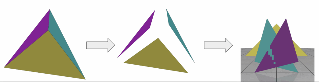
Translation and uniform scaling does not affect the angles, such that we have no angle distortion. So this tells us that this parametrization approach is conformal.
Still, when packing triangles into the texture image, we might need to rescale them so they fit, meaning the areas are not guaranteed to be the same. We can verify this based on the SDF values:
\begin{align*} \sigma_1\sigma_2 \neq 1 \end{align*}This won’t be too relevant in the end though because all triangles get scaled by the same factor, so that the area of each triangle is preserved up to some global scaler. As a result, we would still get an even sampling of the surface, which is what we would care about, at least intuitively, for texture mapping.
However, applying a classical algorithm to trivial parametrization is typically a bad solution because it introduces maximal cuts (discontinuities). How can we overcome this issue?
Parametrization with Neural Networks
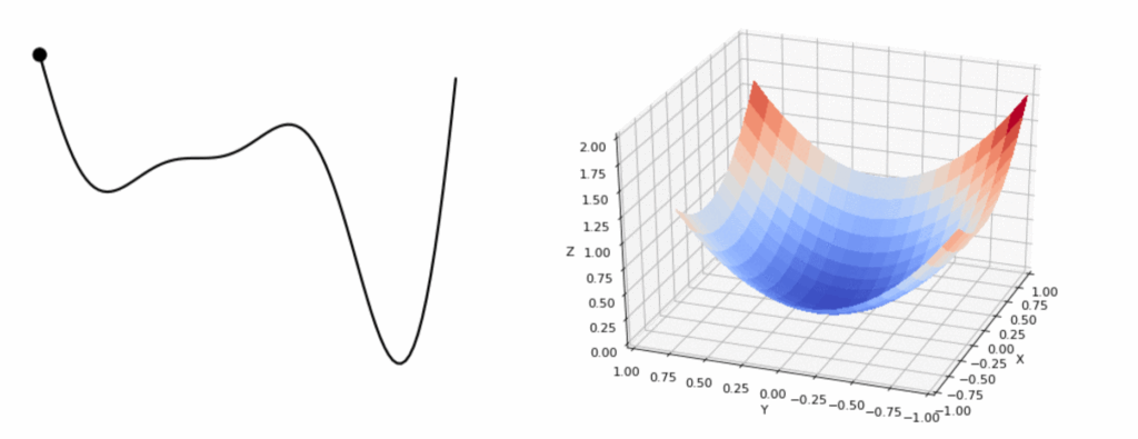
Assume we have some parametrized function and some target value. With an adaptive learning algorithm, we determine the direction in which to change our parameters so that the function moves closer to our target.
We compute some loss or measure of closeness between our current function evaluation and our target value.We then compute the gradient of this loss with respect to our parameters. Take a small step in that direction. We would repeat this process until we ideally achieved the global minimum.
Similarly, we can use an approach to optimize the mesh texture.
- Parametric function = rendering function
- Parameters = texture map pixel values (texel = texture pixel)
- Target = existing images of the object with the desired colors
- Loss = pixel differences between our rendered images and target images.
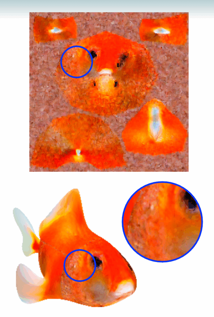
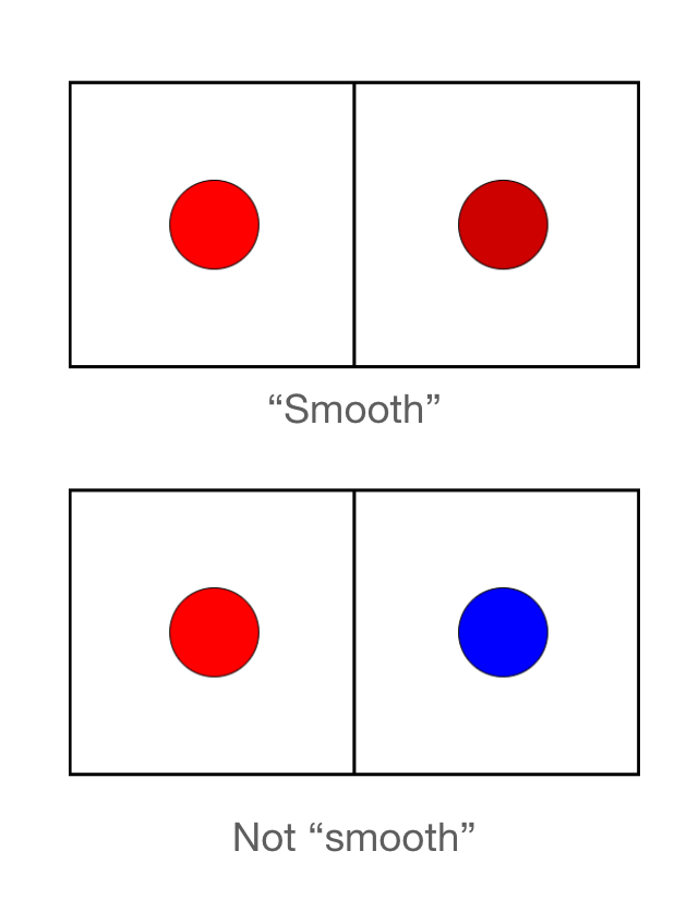
What happens if we do this? We do achieve a texture map, but each pixel is mostly optimized independently. As a result, the texture ends up more grainy.
Improving Smoothness
What can we do to improve this? Well, we would want to make the function more smooth. For this, we can optimize a new function \(\phi(u, v) : \mathbb{R}^2 \rightarrow \mathbb{R}^2\) that maps the texels to RGB color values. By smoothness in \(\phi\), we mean that \(\phi\) is continuous.
To get the color at any point in the 2D texture map, we just need to query \(\phi\) at that UV coordinate!
To encourage smoothness in \(\phi\), we can use a 3D coordinate network.
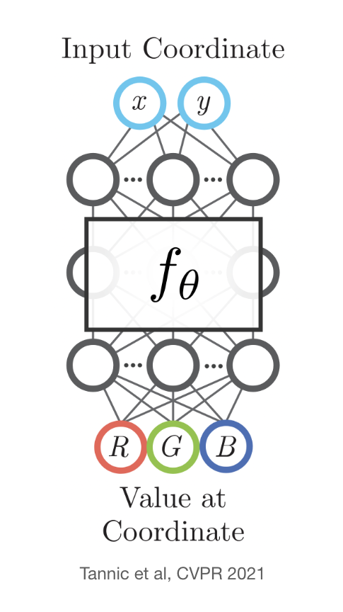
Tannic et al, CVPR 2021
Consider a mapping from a 3D surface to a 2D texture. We can learn a 3D coordinate \(\phi\): \(\mathbb{R}^3 \rightarrow \mathbb{R}^2\) that maps 3D surface points to RGB colors. \(\phi(x, y, z) = (R, G, B)\).
We can then use the inverse map to go from 2D texture coordinates to 3D surface points, then query those points with the coordinate network to get colors, then map those colors back to the 2D texture for easy rendering.
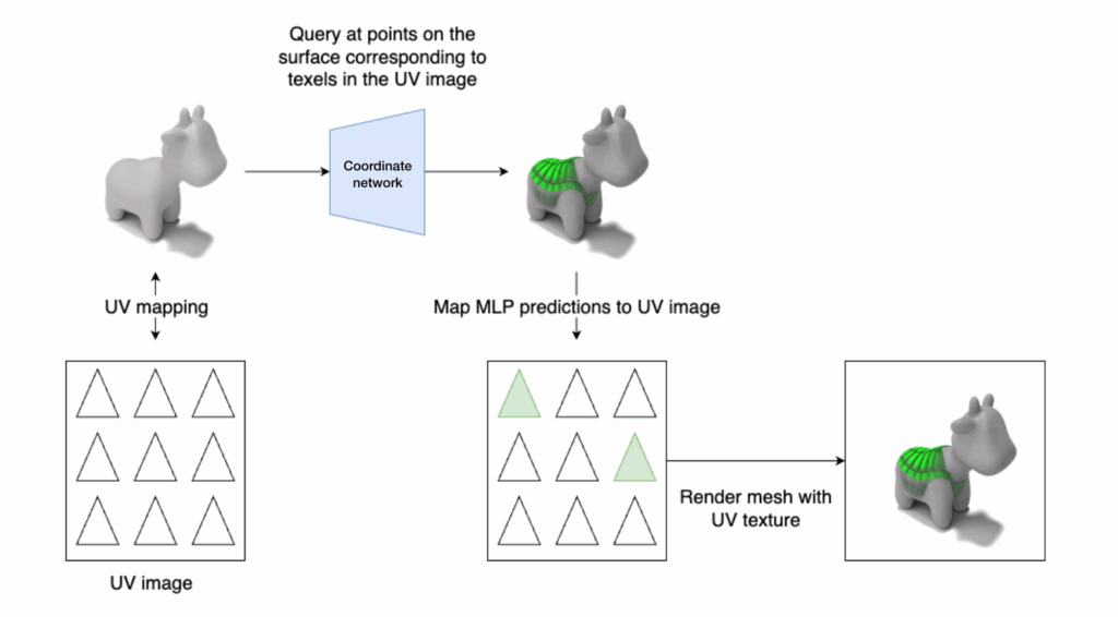
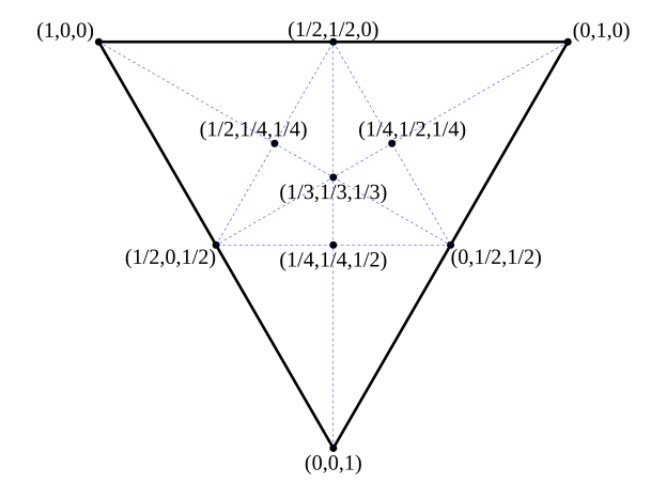
How to compute an inverse map?
We aim to have a mapping from texels to surface poitns, but we already have a mapping from the vertices to the texel plane. The way we can map an arbitrary coordinate to the surface is through barycentric interpolation, a coordinate system relative to a given triangle. In this system, any points has 3 barycentric coordinates.