Categories
research

Neural Implicit Boundary Representations

By SGI Fellow Xinwen Ding and Ahmed Elhag

During the third and fourth week of SGI, Xinwen Ding, Ahmed A. A. Elhag and Miles Silberling-Cook (week 3 only) worked under the guidance of Benjamin Jones and Prof. Adriana Schulz to explore methods that can define a continuous relaxation of CAD geometry.

Background

In general, there are two ways to represent shapes: explicit representations and implicit representations. Explicit representations are easier to model and allow local differentiable parameterizations. CAD geometry, stored in an explicit form called parametric boundary representations (B-reps), is one example, while triangle mesh is another typical example.

However, just as each triangle facet in a triangle mesh has its independent parameterization, it is hard to represent a surface using one single function under an explicit representation. We call this property discrete at the global scale. This discreteness forces us to catch continuous changes using discontinuous shape parameterization and results in weirdness and artifacts. For example, explicit representations can be incompatible with some gradient-based methods and some neural network techniques on a non-local scale.

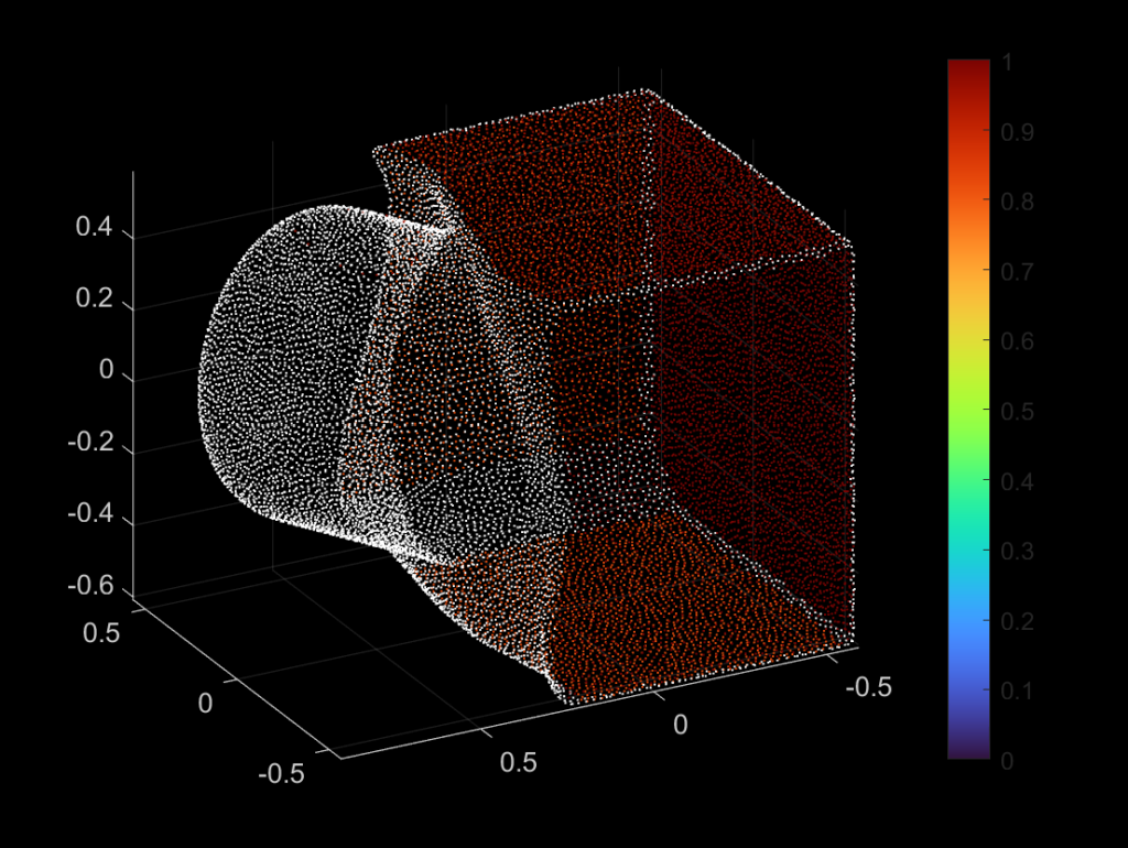
One possible fix to this issue is to use implicit shape representations, such as signed distance field (SDF). SDFs are global functions that are continuously differentiable almost everywhere in the domain, which addresses the issues caused by explicit representations. Motivated by this, we want to play the same trick by defining a continuous relaxation of CAD geometry.

Problem Description

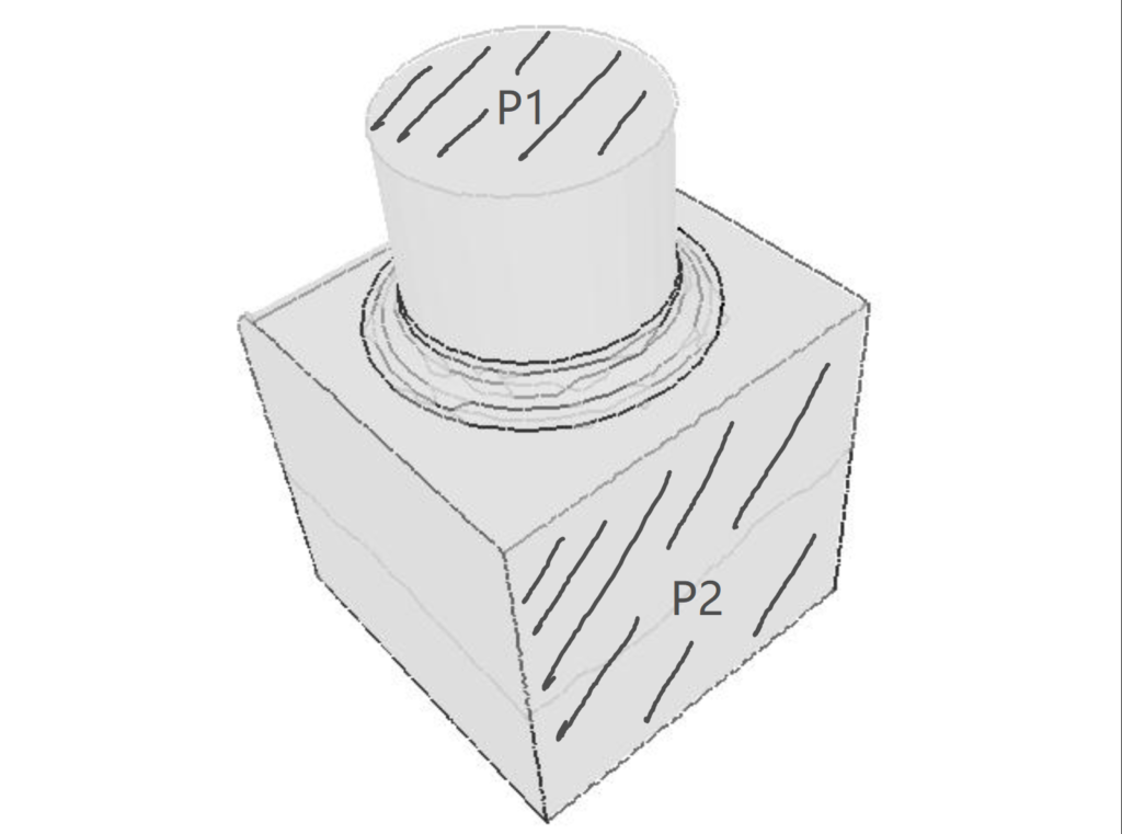
To define this continuous relaxation of CAD geometry, we need to find a continuous relaxation of the boundary element type. Consider a simple case where the CAD data define a geometry that only contains two types; lines and circles. While it is natural that we map lines to 0 and circles to 1,  there is no type defined in the CAD geometry as the pre-image of (0,1). So, we want to define these intermediate states between lines and circles.

The task contains two parts. First, we need to learn the SDF and thus obtain the implicit shape representation of the CAD geometry. As an alignment to the input data type, we want to convert the type-blended geometry to CAD data. So next, we want to convert the SDF back to valid boundary representation by recovering the parameters of the elements we encoded in the SDF and then blending their element type.

The Method

To make it easier for the reconstruction task, we decided to learn multiple SDFs, one for each type of geometry. According to these learned SDFs, we can step into the process of recovering the geometries based on their types. Now, let us consider a concrete example. If we have a CAD shape that consists of two types of geometries, say lines and circles, we need to learn two SDFs: one for edges (part of circles) and another for arcs (part of circles). With these learned SDFs, We hope to recover all the lines that appear in the input shape from the line SDF, and a similar expectation applies to the circle SDF.

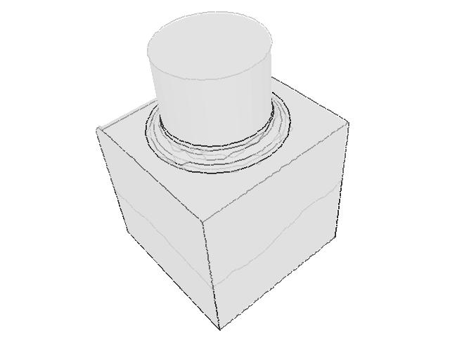
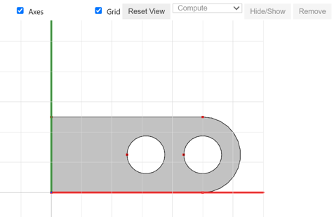
Before jumping into detailed implementations, we want to acknowledge Miles Silberling-Cook for bringing up the multi-SDF idea. Due to the time limitation at SGI, we only tested this method for edges in 2D. We start with the CAD data defining a shape in Figure 1. All the results we show later are based on this geometry.

Figure 1: Input geometry defined by CAD data.

Learned SDF

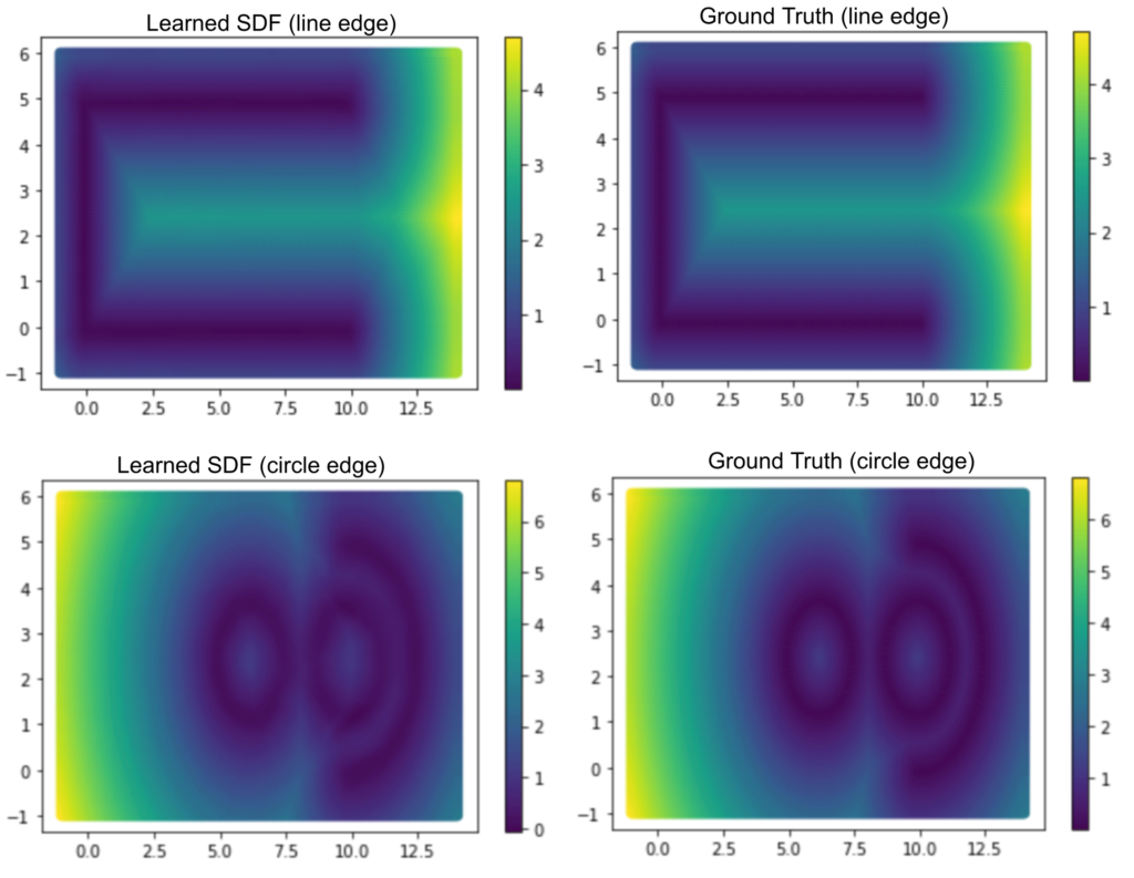
Our goal is to learn a function that maps a coordinate of a query point \((x,y) \in \mathbb{R^2}\) to a signed distance in \(\mathbb{R}\) from \((x,y)\) to the surface. The output of this function is positive if \((x,y)\) is outside the surface, negative if \((x,y)\) is enclosed by the suface, and zero if \((x,y)\) lies on the surface. Thus, our neural network is defined as \(f: \mathbb{R} ^2 \to \mathbb{R}\). For Figure 1, we learned two neural networks, the first network maps \((x,y)\) to its distance from the line edge, and the second network maps this point to its distance for the circle edge.  For this task, we use a Decoder network (multi-layer perceptron, MLP), and optimize it using a gradient descent until convergence. Our dataset was created from a grid with appropriate dimensions, as these are our 2D points. Then, for each point in the grid, we calculate its distance from the line edge and the circle edge.

We compare the image from the learned SDF and the ground truth in Figure 2. It clearly shows that we can overfit and learn both the two networks for line and circle edges.

Figure 2: The network learned the SDF with respect to the edges (first row) and arcs (second row) of the input geometry displayed in Figure 1. We compare the learned result (left column) with the ground truth (right column).

Reconstruction

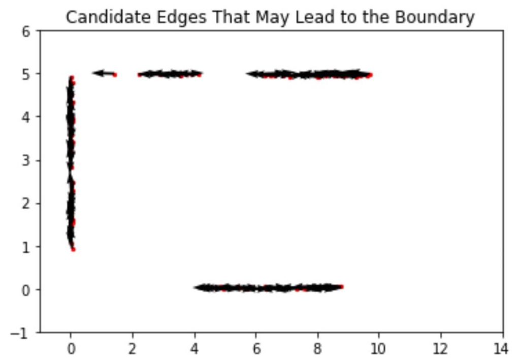
After obtaining the learned line SDF model, we need to analytically recover the edges and arcs. To define an edge, we need nothing but a starting point, a direction, and a length. So, we begin the recovery by randomly seeding thousands of points and assigning each point a random direction. Furthermore, we can only accept those points with their associated values in SDF to be close to zero (see Figure 3), which enhances the success rate of finding an edge as a part of the shape boundary.

Figure 3: we iteratively generate points until 6000 of them are accepted (i.e. SDF value small enough). The accepted points are plotted in red.

Then, we need to tell which lines are more likely to be the ones that define the boundary of our CAD shape and reject the ones that are unlikely to be on the boundary. To guarantee a fair selection, we need to fix the length of the randomly generated edges and pick the ones whose line integral of the learned line SDF is small enough. Moreover, to save more time, we approximate the integral by a finite sum, where we sum up the SDF value assumed by a fixed number of sample points along every edge. Stopping here, we have a pool of edge boundary candidates. We visualize them in terms of their starting points and direction using a quiver plot in Figure 4.

Figure 4: Starting points (red dots) and proper directions (black arrows) that define potential edges.

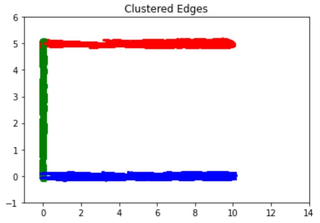
In the next step, we want to extend the candidate edges as long as possible, as our goal is to reconstruct the whole boundary. The extension ends once the SDF value of some extended point exceeds some threshold. After the extension, we cluster the extended edges using the mean shift algorithm. We adopt this clustering algorithm since it does not need to pre-determine the number of clusters. As shown in Figure 5, the algorithm successfully predicts the correct number of edge clusters after carefully tuning the parameters.

Figure 5: Clustered edges. Each color represents one cluster. After carefully tuning parameters, the optimal number of clusters found by the mean shift algorithm reflects the actual number of edges in the geometry.

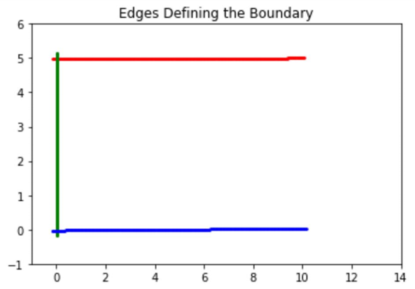
Finally, we want to extract the lines that best define the shape boundary. As we set a threshold in the extension process, we simply need to choose the longest edge from each cluster and name it a boundary edge. The three boundary edges in our example, one in each color, appear in Figure 6.

Figure 6: The longest edges, one from each cluster, with parameters known.

Results

To sum up, during the project’s two-week active period, we managed to complete the following items:

  • We set up a neural network to learn multiple SDFs. The model learns the SDF for edge and arc components on the boundary of a 2D input shape.
  • We developed and implemented a sequence of procedures to reconstruct the lines from the trained line SDF model.

Future Work

Even though we showed the results we achieved during the two weeks, there are more things to improve in the future. First of all, we need to reconstruct the arcs in 2D and ensure the whole procedure to be successful in more complicated 2D geometries. Second, we would like to generalize the whole process to 3D. More importantly, we are interested in establishing a way to smoothly and continuously characterize the shape transfer after the reconstruction. Finally, we need to transfer the continuous shape representation back to a CAD geometry.

Categories
research

Plane and Edge Detection by the Random Sample Consensus (RANSAC)  Algorithm

By SGI Fellows Xinwen Ding, Josue Perez, and Elshadai Tegegn

During the second week of SGI, we worked under the guidance of Prof. Yusuf Sahillioğlu to detect planes and edges from a given point cloud. The main tool we applied to complete this task is the Random Sample Consensus (RANSAC) algorithm.

Definition

We define a plane P as the dominant plane of a 3D point cloud if the number of points defined in the 3D point cloud located on the plane P is no less than the number of points on any other plane. For example, consider the following object defined by a 3D point cloud. If we assume the number of points on a face is proportional to the area of the face, then \(P_2\) is more likely to be the dominant plane than \(P_1\) since the area of \(P_2\) is greater than that of \(P_1\). So, compared with \(P_1\), there are more points on \(P_2\), which makes \(P_2\) the potential dominant plane.

An object that is defined by a point cloud, where P2 is more likely to be the dominant plane than P1.

Problem Description

Given a 3D point cloud as the input model, we aim to detect all the planes in the model. To obtain a decent detection result, we divide the problem into two separate parts:

  • Part 1: Find the dominant plane \(P\) from a given 3D point cloud. This subproblem can be solved by the RANSAC Algorithm.
  • Part 2: Find all other planes contained in the 3D point cloud. This subproblem can be successfully addressed if we iteratively repeat the following two steps: (1). remove all the points on plane \(P\) (obtained from Part 1) from the given point cloud. (2). repeat the RANSAC algorithm with respect to the remaining points in the point cloud.

The RANSAC Algorithm

An Introduction to RANSAC

The RANSAC algorithm is a learning technique that uses random sampling of observed data to best estimate the parameters of a model.
RANSAC divides data into inliers and outliers and yields estimates computed from a minimal set of inliers with the most outstanding support. Each data is used to vote for one or more models. Thus, RANSAC uses a voting scheme.

Workflow & Pseudocode

RANSAC achieves its goal by repeating the following steps:

  • Sample a small random subset of data points and treat them as inliers.
  • Take the potential inliers and compute the model parameters.
  • Score how many data points support the fitting. Points that fit the model well enough are known as the consensus set.
  • Improve the model accordingly.

This procedure repeats a fixed number of times, each time producing a model that is either rejected because of too few points in the consensus set or refined according to the corresponding consensus set size.

The pseudocode of the algorithm is recorded as below:

function dominant_plane = ransac(PC)
    n := number of points defined in point cloud PC

    max_iter := max number of iterations

    eps := threshold value to determine data points that are 
           fit well by model (a 3D plane in our case)

    min_good_fit := number of nearby data points required to 
                    assert that a model (a 3D plane in our 
                    case) fits well to data

    iter := current iteration

    best_err := measure of how well a plane fits a set of 
                points. Initialized with a large number

    % store dominant plane information
    % planes are characterized as [a,b,c,d], where
    % ax + by + cz + d = 0
    dominant_plan = zeros(1,4);

    while iter < max_iter
        maybeInliers := 3 randomly selected values from data 
        maybePlane := a 3D plane fitted to maybeInliers
        alsoInliers := [] 
        for every point in PC not in maybeInliers
            if point_to_model_distance < eps
                add point to alsoInliers
            end if
        end for

        if number of points in alsoInliers is > min_good_fit
            % the model (3D plane) we find is accurate enough

            % this betterModel can be found by solving a least 
            % square problem.
            betterPlane := a better 3D plane fits to all 
                        points in maybeInliers and alsoInliers
            err := sum of distances from the points in 
                   maybeInliers and alsoInliers to betterPlane
            if err < best_err
                best_err := err
                dominant_plane := betterPlane
            end if
        end if

        iter = iter + 1;
    end while
end

Detect More Planes

As mentioned before, to detect more planes, we may simply remove the points that are on the dominant plane \(P\) of the point cloud, according to what is suggested by the RANSAC algorithm. After that, we can reapply the RANSAC algorithm to the remaining points, and we get the second dominant plane, say \(P’\) of the given point cloud. We may repeat the process iteratively and detect the planes one by one until the remaining points cannot form a valid plane in 3D space.

The following code provides a more concrete description of the iterative process.

% read data from .off file
[PC, ~] = readOFF('data/off/330.off');

% A threshold eps is set to decide if a point is on a detected 
% plane. If the distance from a point to a plane is less than 
% this threshold, then we consider the point is on the plane.
eps = 2e-3;

while size(PC, 1) > 3
    % in the implementation of ransac, if the algorithm cannot 
    % detect a plane using the existing points, then the 
    % coefficient of the plane (ax + by + cz + d = 0) is a 
    % zero vector.
    curr_plane_coeff = ransac(PC);
    
    if norm(curr_plane_coeff) == 0
        % remaining points cannot lead to a meaningful plane.
        % exit loop and stop algorithm
        break;
    end

    % At this point, one may add some code to visualize the 
    % detected plane.

    % return the indices of points that are on the dominant
    % plane detected by RANSAC algorithm
    [~, idx] = pts_close_to_plane(PC, curr_plane_coeff, eps);

    % remove the points on the dominant plane.
    V(idx,:) = [];
end

Results

RANSAC algorithm gives good results with 3D point clouds that have planes made up of a good number of points. The full implementation is available on SGI’s Github. This method is not able to detect curves or very small planes. The data we used to generate these examples are the Mechanical objects (Category 17) from this database.

Successful Detections

Mech. Data Model NumberModel Object RANSAC Plane Detection Result
330
331
In the third column, red dots are points on the most dominant plane, followed by blue and green dots are points on the least dominant plane.

Unsuccessful Detections

Mech. Data Model NumberModel Object RANSAC Plane Detection Result
332
338
In the third column, red dots are points on the most dominant plane, followed by blue and green dots are points on the least dominant plane. White points are the ones that cannot be characterized as a plane by the RANSAC algorithm.

Limitations and Future Work

As one may observe from the successful and unsuccessful detections, the RANSAC algorithm is good at detecting planar surfaces. However, the algorithm usually fails to detect a curved surface, because we are fitting the three randomly selected points using a plane equation as our base model. If we change this model to be a curved surface, then theoretically speaking, the RANSAC algorithm should be able to detect a curved plane. We may apply a similar fix if we want to perform line detection.

Moreover, we may notice that the majority of surfaces in our test data can be represented easily by an analytical formula. However, this pre-condition is, in general, not true if we choose an arbitrary point cloud. If this is the case, the RANSAC algorithm is unlikely to output an accurate detection result, which leads to more extra work.

Categories
tutorial week

A Summary of the Shape Deformation Lecture with an Example

By SGI Fellows Xinwen Ding and Miles Silberling-Cook

The authors of this article appreciate Derek Liu and Eris Zhang for their awesome lectures on the third day of SGI. The rest of this summary is based on what we learned from their lectures.

Introduction

One of the motivations for shape deformation is the desire of reproducing the motion of a given initial shape as time evolves. It is clear that modeling every piece of information associated with the initial shape can be hard and unnecessary. So, a simple but nice-looking deformation strategy is needed. During the lecture, SGI fellows were introduced two deformation strategies listed below.

  • Energy-based Deformation: This method turns the deformation problem into an optimization problem, where possible objective functions can be Dirichlet Energy (\(E = \int_{M} ||\nabla f||^2 dx\)), Laplacian Energy (\(E = \int_{M} ||\Delta f||^2 dx\)), or Conformal Energy. It is worth mentioning that the nonlinear optimization problems are, in general, difficult to solve.
  • Direct Method: We mainly refer to a method called Linear Blend Skinning (LBS). In this method, we predefine a sequence of movable handles. Furthermore, we assume the movement of every handle will contribute linearly to the final coordinate of our input vertex. Based on this assumption, we write down the equation for calculating the target position: \(u_i = \displaystyle\sum_{j = 1}^{\text{# of handles}} w_{ij} T_j v_i\), where \(v_i, u_i\) are the \(i^{th}\) input and output vertices, respectively, \(w_{ij}\) is the weight, and \(T_j\) is the tranformation matrix of the \(j^{th}\) handle recording rotation and transformation in terms of homogeneous coordinates.

The remaining part of this summary will focus on the Linear Blend Skinning (LBS) method.

Workflow

The process of a 2D LBS deformation can be divided into three steps:

  • Step 1: Define the handles.
  • Step 2: Compute the weights \(w_{ij}\) and store the tranformation matrix \(T_j = \begin{bmatrix}\cos\theta & -\sin\theta & \Delta x \\ \sin\theta & \cos\theta & \Delta y\end{bmatrix}\), where the first two columns of \(T_j\) denote the rotation of the \(j^{th}\) handle, and the last column denotes the shift. Notice that in this case the \(i^{th}\) vertex should be \(v_i = \begin{bmatrix} v_x \\ v_y \\ 1\end{bmatrix}\).
  • Step 3: Put all parts together and compute \(u_i = \displaystyle\sum_{j = 1}^{\text{# of handles}} w_{ij} T_j v_i\).

A concrete example will be given in the final section.

Weight Calculation

Requirements on weights:

To minimize the artifacts in our deformation, we need to be smart when we generate the weights. Briefly speaking, we want our weights to satisfy the following criteria:

  • Smooth: the weight function should be \(C^{1}\) differentiable. This can be achieved by introducting the Laplacian operator.
  • Local: the effective area in a 2D domain should be within some neighborhood of the handle.
  • Shape aware: the effective area in a 2D domain should not cross the boundary of our domain of interest.
  • Sum up to 1.

Let \(\Omega\) be the domain of the interest, and \(w\) be the weight. Based on the aforementioned requirements, we can use the following minimization problem to characterize the weights.

\begin{equation}
\begin{aligned}
&\min_{w} \int_{\Omega} || \Delta w||^2 dx \\
&\textrm{s.t.} w(j^{th} \text{handle}) = e_j \hspace{20pt} \text{($e_j$ is a standard basis vector)}
\end{aligned}
\end{equation}

Discretize the Laplacian Operator

One may notice that in the objective function of the above optimization problem, we introduced a Laplacian operator. Luckily, we can play some math tricks to discretize the Laplacian operator, namely \(\Delta = M^{-1}C\), where \(M\) is the diagonal mass matrix, and \(C\) is the cotangent formula for the Laplacian.

With this knowledge in mind and with some knowledge from Finite Element Method, we can rewrite the objective function into a quadratic form.

\[
\int_{\Omega} || \Delta w||^2 dx
= ||M^{-1}Cw||_{M}^2
= (M^{-1} C w)^{T} M (M^{-1} C w)
= w^{T} C^{T} M^{-1} C w
\]

Let \(B = C^{T} M^{-1} C\), then we have \(\int_{\Omega} || \Delta w||^2 dx = w^{T} C^{T} M^{-1} C w = w^{T} B w\). Moreoever, we name the matrix \(B\) as bilaplacian or square Laplacian. Hence, the optimization problem is rewritten as follows:

\begin{equation}
\begin{aligned}
&\min_{w} w^{T} B w \\
&\textrm{s.t.} w(j^{th} \text{handle}) = e_j \hspace{20pt} \text{($e_j$ is a standard basis vector)}
\end{aligned}
\end{equation}

Solution Derivation to the Optimization Problem

Recall that \(w_{ij}\) is the degree to which vertex \(i\) is effected the motion of handle \(j\). To form our constraint, we pick a vertex for each handle that will only be affected by that handle. This constraint is much easier to express when the fixed weightings are separated from the free weightings, so we re-organize the weightings as \(w = [x, y]\). In this notation, \(x\) contains the free variables for the non-handle vertices, and \(y\) contains the fixed weighting for each handle. The boundary can now be concisely stated as \(y = \mathbb{I}\).

We now solve for the \(x\) that minimizes \([x \mid y]^T B [x \mid y]\). Following Derek Liu and Eris Zhang’s lead, we use subscripts to express the indices of \(B\) pertaining to either \(x\) or \(y\).

\begin{align}
E
&= w^T B w \\
&= [x \mid y]^T B [x \mid y] \\
&= [x \mid 0]^T \begin{bmatrix}B_{x,x} & 0 \\ 0 & 0 \end{bmatrix} [x \mid 0]
+ [x \mid 0]^T \begin{bmatrix}0 & B_{x,y} \\ 0 & 0 \end{bmatrix} [0 \mid y]
+ [0 \mid y]^T \begin{bmatrix}0 & 0 \\ B_{y,x} & 0 \end{bmatrix} [x \mid 0]
+ [0 \mid y]^T \begin{bmatrix}0 & 0 \\ 0 & B_{y,x} \end{bmatrix} [0 \mid y] \\
&= x^T B_{x,x} x + x^T B_{x,y} y + y^T B_{y,x} x + y^T B_{y,y} y \\
&=
\underbrace{ x^T B_{x,x} x }_\text{Quadratic}
+ \underbrace{ x^T \left(B_{x,y} + B_{y,x}^T \right) y }_\text{Linear}
+ \underbrace{ y^T B_{y,y} y }_\text{Constant}
\end{align}

As expected, this yields another quadratic equation. Differentiating gives:

\begin{equation}
\frac{\partial E}{\partial x}
= 2 A_{x,x,} x + \left(B_{x,y} + B_{y,x}^T \right) y
\end{equation}

and the extremizer is therefore \(x = \left( -2A\right)^{-1}\left(B_{x,y} + B_{y,x}^T \right) y\).

Code Implementation and Acceleration

Implementation

To calculate the solution in Matlab, see the following.

function W = compute_skinning_weight(V,F,b)
% V: Vertices
% F: Triangles
% b: Handle vertex indices

% Compute the Laplacian using the cotangent-matrix.
L = -cotmatrix(V,F);

% Compute the mass matrix.
M = massmatrix(V,F);

% Compute the BiLaplacian
B = L*(M\L);

% Create a list of non-handle verticies
a = setdiff(1:size(V,1), b);

% Initialize the fixed handle constraint
y = eye(length(b));

% Compute the minimum
A = Q(a,a);
B = (Q(a,b) + Q(b,a).') * y;
x = (-2*A) \ B;

% Assemble the final weight matrix
W(a,:) = x;
W(b,:) = y;
end

Once the weightings are done, we can propagate the transformation of the handles to the mesh (using homogeneous coordinates) as follows:

function [U] = linear_blend_skinning(V, T, W)
% V: Vertices
% T: Handle transforms
% W: Weighting matrix

U = zeros(size(V));

for i=1:size(V)

for j=1:size(T,3)
U(i,:) = U(i,:) + ( W(i,j) * [V(i,:) 1] * T(:,:,j).' );
end

end

end

Acceleration

Although the solution above guarantees correctness, this is a fairly inefficient implementation. Some of this computation can be done offline, and the nested loops are not required. The blending weights and the vertex positions can be compiled into a single matrix ahead of time, like so:

function C = compile_blending_weights(V, N, W)
% V: Vertices
% N: Number of handles
% W: Weighting matrix

for i=1:length(V)
v = repmat( [V(i,:), 1], 1, N)';
wi = reshape(repmat(W(i, :), 3, 1), [], 1);
C(:,i) = v.*wi;
end
end

Then propagating the transform is as simple as composing it with the precomputed weightings.

function [U] = linear_blend_skinning(T, C)
% T: Handle transforms
% C: Compiled blending weights

B = reshape(T,[], size(T, 3)*size(T, 2));
U = (B*C)';
end

Shout-out to SGI Fellow Dimitry Kachkovski for providing this extra-efficient implementation!

Example: 2D Gingerbread Man Deformation

In this example, we try to implement the whole method over a gingerbread man domain. Following the define handle – computing weights – combine and transform workflow, we provide a series of video examples.

Step 1: Define handles

By click randonly on the mesh, the handles are defined according to the position of mouse.

Step 2: Computing Weights

The area where the weight function is effective is in some color other than blue.

Step 3: Combine and Transform

Drag the handles and deform the gingerbread man!