Using Gray-Scott Reaction-Diffusion Model to Create Spots (and Stripes) on 3D Spot

By SGI Fellow Natalie Patten

The Gray-Scott reaction-diffusion model consists of two partial differential equations: $$\frac{\partial U}{\partial t}=D_u\nabla^2U-UV^2+F(1-U)$$ $$\frac{\partial V}{\partial t}=D_v\nabla^2V+UV^2-(F+k)V.$$Using a semi-implicit approach, each \(U^{i+1}\) can be calculated as follows: \((I -{\Delta}tD_uL)U^{i+1}=U^i + {\Delta}t (F(1-U^i) – U^iV^iV^i)\). Here, \(I\) is the identity matrix, \({\Delta}t\) is change in time, \(D_u\) is the diffusion rate, \(L\) is the Laplacian of the mesh, \(F\) is the feed rate, and \(k\) is the degrading rate. Similarly, \(V^{i+1}\) can be calculated as follows: \((I -{\Delta}tD_vL)V^{i+1}=V^i + {\Delta}t (U^iV^iV^i-(F+k)V^i)\). Using Eigen‘s SimplicialLDLT solver, which uses Cholesky decomposition, we can solve for each:

Eigen::SparseMatrix<double> temp1 = (I - timeStep * du * L).eval();
Eigen::SparseMatrix<double> temp2 = (I - timeStep * dv * L).eval();

Eigen::SimplicialLDLT<Eigen::SparseMatrix<double>> solver1;
Eigen::SimplicialLDLT<Eigen::SparseMatrix<double>> solver2;

solver1.compute(temp1);
solver2.compute(temp2);

for (int i = 0; i < numSteps; i++) {
   Eigen::VectorXd UVV = U.array() * V.array() * V.array();
   Eigen::VectorXd FU = F.array() * U.array();
   U = solver1.solve((U + timeStep * (F - FU - UVV)).eval());
   Eigen::VectorXd kV = k.array() * V.array();
   Eigen::VectorXd FV = F.array() * V.array();
   V = solver2.solve((V + timeStep * (UVV - kV - FV)).eval());
}

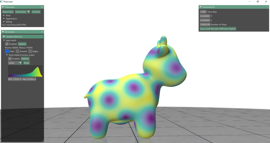
U was initialized to be 1.0 everywhere, and V was initialized to be 0.0 everywhere except in one small area where it was initialized to be 1.0. D_u and D_v were set to be 1.0 and 0.5, respectively. I then modelled this onto a 3D mesh of Spot the cow using Polyscope with a time step of 1 and various F and k values, based on parameters found in Pearson’s “Complex Patterns in a Simple System” (1993). Below is a summary of the initial results. You can see various patterns formed by the Gray-Scott model.

F = 0.024 and k = 0.06 at 10,000 steps:

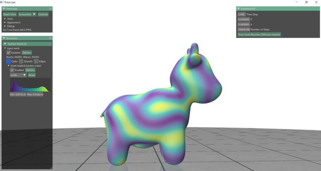
F = 0.04 and k = 0.06 at 10,000 steps:

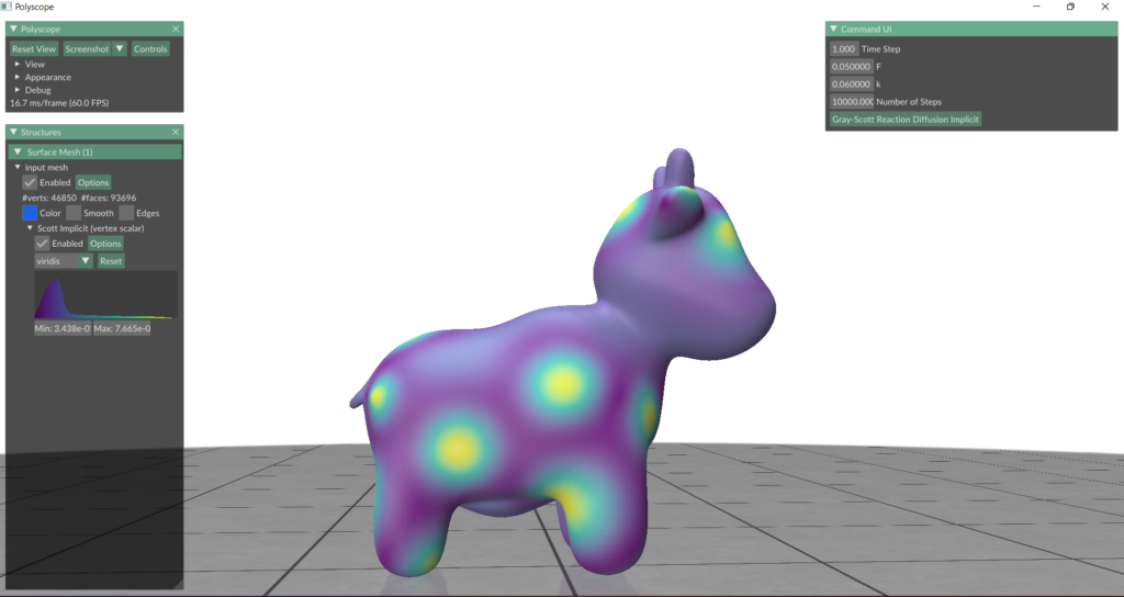
F = 0.05 and k = 0.06 at 10,000 steps:

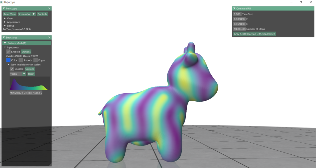
F = 0.03 and k = 0.056 at 10,000 steps:

F = 0.044 and k = 0.063 at 10,000 steps:

Acknowledgments:

• Thank you to my project partners Mariem Khlifi and Gimin Nam for help with (lots of!) debugging.
• Thank you to my project mentor Etienne Vouga and project TA Erick Jimenez Berumen for guidance, debugging, and resources.