Hi! I am Brittney Fahnestock, and I am a rising senior at the State University of New York at Oswego. This is one of the smaller, less STEM-based state schools in New York. That being said, I am a mathematics education and mathematics double major. Most of my curriculum has been pedagogy-based, teaching mathematics and pure mathematics topics like algebraic topology.
So, as you might have read, that does not seem to have applied mathematics, coding, or geometry processing experience. If you are thinking that, you are right! I have minimal experience with Python, PyTorch, and Java. All of my experience is either based on statistical data modeling or drawing cute pictures in Java. So again, my experience has not been much help with what was about to take place!
The introduction week was amazing, but hard. It helped me catch up information-wise since I had minimal experience with geometry processing. However, the exercises were time-consuming and challenging. While I felt like I understood the math during the lectures, coding up that math was another challenge. The exercise helped to make all of the concepts that were lectured about more concrete. While I did not get them all working perfectly, the reward was in trying and thinking about how I could get them to work or how to improve my code.
Now, onto what my experience was like during the research! In the first week, we worked with Python. I did a lot more of the coding than expected. I felt lost many times with what to do, but in our group, we were trying to get out of our comfort zones. Getting out of our comfort zones allows us to grow as researchers and as humans. As a way to make sure we were productive, we did partner coding. My partner knew a lot more about coding than I did. This was a great way to learn more about the topic with guidance!
We worked with splines, which of course was new for me, but they were interesting. Splines not only taught me about coding and geometry but also the continuity of curves and surfaces. The continuity was my favorite part. We watched a video explaining how important it is for there to be strong levels of continuity for video games, especially when the surfaces are reflective.
Week two was a complete change of pace. The language used was C++, but no one in the group had any experience with C++. Our mentor decided that we would guide him with the math and coding, but he would worry about the syntax specifics of C++. I guess this was another form of partner/group coding. While it exposed us to C++, our week was aimed at helping us understand the topics and allowing us to explore what we found interesting.
We worked with triangle marching and extracting iso-values with iso-segmentation and simplices. I had worked with simplicies in an algebraic topology context and found it super interesting to see the overlap in the two fields.
I have an interest in photography, so the whole week I saw strong connections to a passion of mine. This helped me to think of new questions and research ideas. While a week was not quite long enough to accomplish our goal, we plan on meeting after SGI to continue our work!
I can not wait for the last three weeks of SGI so I can continue to learn new ideas about geometry processing and research!
For the past two weeks, our project team mentored by Dr. Ankita Shukla set out to understand the inner workings of OpenAI’s CLIP model. Specifically, we were interested in gaining a mathematical understanding of feature spaces’ geometric and topological properties.
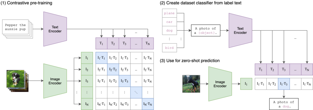
OpenAI’s CLIP (Contrastive Language-Image Pre-Training) is a versatile and powerful model designed to understand and generate text and images. CLIP is trained to connect text and images by learning from a large dataset of images paired with their corresponding textual descriptions. The model is trained using a contrastive learning approach, where it learns to predict which text snippet is associated with which image from a set of possible pairs. This allows CLIP to understand the relationship between textual and visual information.
Figure 1: OpenAI’s CLIP architecture as it appears in the paper. CLIP pre-trains an image encoder and a text encoder to predict which images were paired with which texts in our dataset. Then OpenAI uses this behavior to turn CLIP into a zero-shot classifier. We convert all of a dataset’s classes into captions such as “a photo of a dog” and predict the class of the caption CLIP estimates best pairs with a given image.
CLIP uses two separate encoders: a text encoder (based on the Transformer architecture) and an image encoder (based on a convolutional neural network or a vision transformer). Both encoders produce embeddings in a shared latent space (also called a feature space). By aligning text and image embeddings in the same space, CLIP can perform tasks that require cross-modal understanding, such as image captioning, image classification with natural language labels, and more.
CLIP is trained on a vast dataset containing 400 million image-text pairs collected online. This extensive training data allows it to generalize across various domains and tasks. One of CLIP’s standout features is its ability to perform zero-shot learning. It can handle new tasks without requiring task-specific training data, simply by understanding the task description in natural language. More information can be found in OpenAI’s paper.
In our attempts to understand the inner workings of the feature spaces, we employed tools from UMAP, persistence homology, subspace angles, cosine similarity matrices, and Wasserstein distances.
Our Study – Methodology and Results
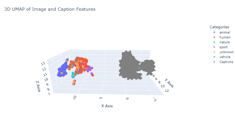
All of our teammates started with datasets that contained image-caption pairs. We classified images into various categories using their captions and embedded them using CLIP. Then we used UMAP or t-SNE plots to visualize their characteristics.
Figure 2: A screenshot of a UMAP of 1000 images from the Flickr 8k dataset from Kaggle divided into five categories (animal, human, sport, nature, and vehicle) is shown. Here we can also observe that the images (colored) are embedded differently than their corresponding captions (gray). Although not shown here, the captions are also clustered around categories.
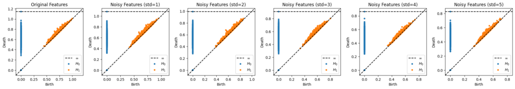
After this preliminary visualization, we desire to delve deeper. We introduced noise, a Gaussian blur, to our images to test CLIP’s robustness. We added the noise in increments (for example mean = 0, standard deviation = {1,2,3,4,5}) and encoded them as we did the original image-caption pairs. We then made persistence diagrams using ripser. We also followed the same procedure within the various categories to understand how noise impacts not only the overall space but also their respective subspaces. These diagrams for the five categories from the Flickr 8k dataset can be found in this Google Colab notebook.
Figure 3: The same 1000 images from the Flickr 8k dataset with increasing noise are seen above. Visually, no significant difference can be observed. The standard deviation of the Gaussian blur increases from left to right.
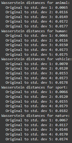
Visually, you can observe that there is no significant difference, which attests to CLIP’s robustness. However, visual assurance is not enough. Thus, we used Scipy’sWasserstein’s distance calculation to note how different each persistence diagram is from the other. Continuing the same Flickr 8k dataset, for each category, we obtain the values shown in Figure 4.
Figure 4: Wasserstein distances in each category. You can see the distance between original images with respect to images with Gaussian blur of std. dev = 1 is not high compared to std. dev = 2 or above. This implies that the original set is not as different from the set of images blurred with std. dev. = 1 as compared to std. dev. = 2 which in turn is not as different as the set of blurred images with std. dev. = 3, and so on. This property holds for all five categories.
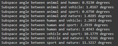
Another question to understand is how similar are each of the categories to one another. This question can be answered by calculating the subspace angles. After embedding, each category can be seen as occupying a space that can often be far away from another category’s space– we want to quantify how far away, so we use subspace angles. Results for the Flickr 8k dataset example are shown in Figure 5.
Figure 5: Subspace angles of each category pair in the five categories introduced earlier in the post. All values are displayed in degrees. You can observe that the angle between human- and animal-category images is ~0.92° compared to human and nature: ~2.3°; which makes sense as humans and animals are more similar than humans compared to nature. It is worthwhile to note that the five categories are simplifying the dataset too much as they do not capture the nuances of the captions. More categories or descriptions of categories would lead to higher accuracy in the quantity of the subspace angle.
Conclusion
At the start, our team members were novices in the CLIP model, but we concluded as lesser novices. Through the two weeks, Dr. Shukla supported us and enabled us to understand the inner workings of the CLIP model. It is certainly thrilling to observe how AI around us is constantly evolving, but at the heart of it is mathematics governing the change. We are excited to possibly explore further and perform more analyses.
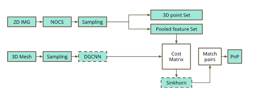
Image 1: Our proposed solution’s pipeline, credits to our -always supportive- mentors, Saleh Mahdi and Dani Velikova!
Introduction
Our project aims to enhance Optimal Transport (OT) solvers by incorporating Graph Neural Networks (GNNs) to address the lack of geometric consistency in feature matching. The main motivation of our study is that a lot of real objects are symmetric and thus impose ambiguity. Traditional OT approaches focus on similarity measures and often neglect important neighboring information in geometric settings, proper in computer vision or graphics problems, resulting in the production of huge noise in pose estimation tasks. To tackle this problem, we hypothetize that when the object is symmetric, there are many correct matches of points around its symmetric axis and we can leverage this fact via Optimal Transport and Graph Learning.
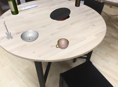
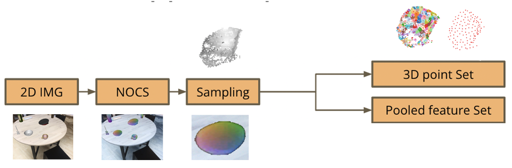
To this end, we propose the pipeline in image 1. On a high level, we extract a 3D point cloud of an object from a 2D scene using the Normalized Object Coordinate Space (NOCs) pipeline [1], downsample the points and pool the features/NOCs embeddings of the removed points into the representative remaining points. Concurrently, we run DGCNN on the 3D ground truth mesh of the object and create a graph; this model is used as a 3D encoder [2]. We combine the aforementioned embeddings into the cost matrix used by the Sinkhorn algorithm [3], which attempts to match the points of the point cloud produced by the NOCs map with the nodes of the graph produced by the DGCNN and then to provide a symmetry estimation. We extend the differentiable Sinkhorn solver to yield one-to-many solutions; a modification we make to fully capture the symmetry of a texture-less object. In the final step, we match pairs of points and pixels and perform symmetric pose estimation via Perspective-n-Point. In this post, we study one part of our proposed pipeline, the extended NOCs, from the 2D image analysis to the extraction of the 3D point set and the pooled feature set.
Extended NOCs pipeline
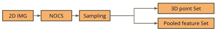
Image 2: The part of the pipeline we will study in this post: Generating a 3D point cloud of a shape from a chosen 2D scene and downsampling its points. We pool the features of the removed points into remaining (seed) points.
The NOCs pipeline extracts the NOCs map and provides size and pose estimation for each object in the scene. The NOCs map encodes via colours the prediction of the normalized 3D coordinates of the target objects’ surfaces within a bounded unit cube. We extend the NOCs pipeline to create a 3D point cloud of the target object using the extracted NOCs map. We then downsample the point cloud, by fragmenting it using the Farthest Point Sampling (FPS) algorithm and only keeping the resulting seed points. In order to fully encapsulate the information extracted by the NOCs pipeline, we pool the embeddings of the nodes of each fragment into the seed points, by averaging them. This enables our pipeline to leverage the features of the target object’s 2D partial view in its scene.
Data
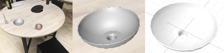
Images 3, 4, 5: (3) The scene of the selected symmetric and texture-less object. (4) The object in the scene zoomed in. (5) The ground truth of the object, i.e. its exact 3D model.
In order to test our hypothesis, we use an object that is not only symmetric, but also texture-less and pattern-free. The specifications of the object we use are the following:
Link to download: https://github.com/sahithchada/NOCS_PyTorch?tab=readme-ov-file
Extended NOCs pipeline: steps visualised
In this section we visually examine each part of the pipeline and how it processes the target shape. First, we get a 2D image of a 3D scene, which is the input of the NOCs pipeline:
Image 6: The 3D scene to be analyzed.
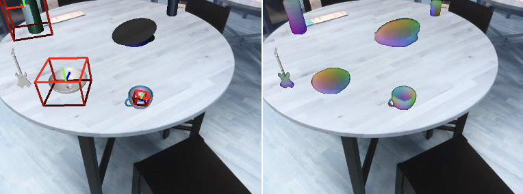
Running the NOCs pipeline on it, we get the pose and size estimation, as well as the NOCs map for every object in the scene:
Image 7, 8: (7) Pose and size estimation of the objects in the scene. (8) NOCs maps of the objects.
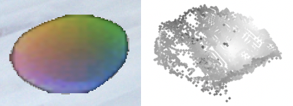
The color encodings in the NOCs map encode the prediction of the normalized 3D coordinates of the target objects’ surfaces, within a bounded a unit cube. We leverage this prediction to reconstruct the 3D point cloud of our target shape, from its 2D representation in the scene. We used a statistical outlier removal method to refine the point cloud and remove noisy points. We got the following result:
Images 9, 10: (9) The 2D NOCs map of the object. (10) The 3D point cloud reconstruction of the 2D NOCs map of the target object.
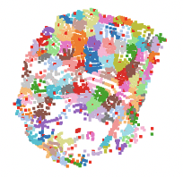
The extracted 3D point cloud of the target object is then fragmented using the Farthest Point Sampling (FPS) algorithm and the seed (center/representative) points of each fragment are also calculated.
Image 11: The fragmented point cloud of the target object. Each fragment contains its corresponding seed point.
The Sinkhorn algorithm part of our project requires a lot less data points for an optimized performance. Thus, we downsample the 3D point cloud, by only keeping the seed points. In order to capture the information extracted by the NOCs pipeline, we pool the embeddings of the removed features into their corresponding seed points via averaging:
Image 12: The 3D seed point cloud. Into each seed point, we have pooled the embeddings of the removed points of their corresponding fragment.
An overview of each step and the visualised result can be seen below:
Image 13: The scene and object’s visualisation across every step of the pipeline.
Conclusion
In this study, we discussed the information extraction of a 3D object from a 2D scene. In our case, we examined the case of a symmetric object. We downsampled the resulting 3D point cloud in order for it to be effectively handled by later stages of the pipeline, but we made share to encapsulate the features of the removed points via pooling. It will be very interesting to see how every part of the pipeline comes together to predict symmetry!
At this point, I would like to thank our mentors Mahdi Saleh and Dani Velikova, as well as Matheus Araujo for their continuous support and understanding! I started as a complete beginner to these computer vision tasks, but I feel much more confident and intrigued by this domain!
[1] He Wang, Srinath Sridhar, Jingwei Huang, Julien Valentin, Shuran Song, and Leonidas J. Guibas. Normalized object coordinate space for category-level 6d object pose and size estimation, 2019. [2] Yue Wang, Yongbin Sun, Ziwei Liu, Sanjay E. Sarma, Michael M. Bronstein, and Justin M. Solomon. Dynamic graph cnn for learning on point clouds, 2019. [3] Paul-Edouard Sarlin, Daniel DeTone, Tomasz Malisiewicz, and Andrew Rabinovich. Superglue: Learning feature matching with graph neural networks. CoRR, abs/1911.11763, 2019.
Two fundamental mathematical approaches to describing a shape (space) \(M\) involve addressing the following questions:
🤔 (Topological) How many holes are present in \(M\)?
🧐 (Geometrical) What is the curvature of \(M\)?
To address the first question, our space \(M\) is considered solely in terms of its topology without any additional structure. For the second question, however, \(M\) is assumed to be a Riemannian manifold—a smooth manifold equipped with a Riemannian metric, which is an inner product defined at each point. This category includes surfaces as we commonly understand them. This note aims to demystify Riemannian curvature, connecting it to the more familiar concept of curvature.
… Notoriously Difficult…
Riemannian curvature, a formidable name, frequently appears in literatures when digging into geometry. Fields Medalist Cédric Villani in his Optimal Transport said
“it is notoriously difficult, even for specialists, to get some understanding of its meaning.” (p.357)
Riemannian curvature is the father of curvatures we saw in our SGI tutorial and other curvatures. In the most abstract sense, Riemann curvature tensor is defined as a \((0,4)\) tensor field obtained by lowering the contravariant index of the \((1,3)\) tensor field defined as
“It also helps to see pictures of surfaces with zero mean and Gaussian curvature. Zero-curvature surfaces are so well-studied in mathematics that they have special names. Surfaces with zero Gaussian curvature are called developable surfaces because they can be ‘developed’ or flattened out into the plane without any stretching or tearing. For instance, any piece of a cylinder is developable since one of the principal curvatures is zero:” (p.39)
Te following video continues with this cylinder example to show difficulties characterizing flatness. It examines the following question: how to use a piece of flat white paper to roll into a doughnut-shaped object (Torus) without distorting the length of the paper. That is, we are not allowed to use a piece of stretchable rubber to do this job.
This is part of an ongoing project. In fact, in an upcoming SIGGRAPH paper “Repulsive Shells” by Prof. Crane and others, more examples of isometric embeddings, including the flat torus, are discussed.
First definition of flatness
A Riemannian \(n\)-manifold is said to be flat if it is locally isometric to Euclidean space, that is, if every point has a neighborhood that is isometric (distance-preserving) to an open set in \(\mathbb{R}^n\) with its Euclidean metric.
Example: flat torus
We denote the n-dimensional torus as \(\mathbb{T}^n=\mathbb{S}^1\times \cdots\times \mathbb{S}^1\), regarded as the subset of \(\mathbb{R}^{2n}\) defined by \((x^1)^2+(x^2)^2+\cdots+(x^{2n-1})^2+(x^{2n})^2=1\). The smooth covering map \(X: \mathbb{R}^n \rightarrow \mathbb{T}^n\), defined by \(X(u^1,\cdots,u^{n})=(\cos u^1,\sin u^1,\cdots,\cos u^n,\sin u^n)\), restricts to a smooth local parametrization on any sufficiently small open subset of \(\mathbb{R}^n\), and the induced metric is equal to the Euclidean metric in \(\left(u^i\right)\) coordinates, and therefore the induced metric on \(\mathbb{T}^n\) is flat. This is called the Flat torus.
Parallel Transport
We still didn’t answer the question why we need four vector fields to characterize how curved a shape is. We will do this by using another useful tool in differential and discrete geometry to view flatness and thus curvedness. We follow John Lee’s Introduction to Riemannian Manifold for this section, first defining the Euclidean connection.
Consider a smooth curve \(\gamma: I \rightarrow \mathbb{R}^n\), written in standard coordinates as \(\gamma(t)=\left(\gamma^1(t), \ldots, \gamma^n(t)\right)\). Recall from calculus that its velocity is given by \(\gamma'(t)=(\dot{\gamma}^1(t),\cdots,\dot{\gamma}^n(t))\) and its acceleration is given by \(\gamma”(t)=(\ddot{\gamma}^1(t),\cdots,\ddot{\gamma}^n(t))\). A curve \(\gamma\) in \(\mathbb{R}^n\) is a straight line if and only if \(\gamma^{\prime \prime}(t) \equiv 0\). Directional derivatives of scalar-valued functions are well understood in our calculus class. Analogs for vector-valued functions, or vector fields, on \(\mathbb{R}^n\) can be computed using ordinary directional derivatives of component functions in standard coordinates. Given a vector \(v\) tangent to \(M\), we define the Euclidean directional derivative of vector field \(Y\) in the direction \(v\) by:
where for each \(i\), \(v(Y^i)\) is the result of applying the vector \(v\) to the function \(Y^i\): $$ v(Y^i) = v^1 \frac{\partial Y^i(p)}{\partial x^1} + \cdots + v^n \frac{\partial Y^i(p)}{\partial x^n}. $$
If \(X\) is another vector field on \(\mathbb{R}^n\), we obtain a new vector field \(\bar{\nabla} _X Y\) by evaluating \(\bar{\nabla} _{X_p} Y\) at each point: $$ \bar{\nabla}_X Y = X(Y^1) \frac{\partial}{\partial x^1} + \cdots + X(Y^n) \frac{\partial}{\partial x^n}. $$
This formula defines the Euclidean connection, generalizing the concept of directional derivatives to vector fields. This notion can be generalized to more abstract connections on \(M\). When we say we parallel transport a tangent vector \(v\) along a curve \(\gamma\), we simply mean picking vectors for each point on the curve that are tagent to the curve and are parallel to each other at the same time. The mathematical way of saying vectors are parallel is to say the derivative of the vector field formed by them are zero (we have just defined the derivatives for vector field above). Let \(T_pM\) denote the set of all vectors tangent to \(M\) at point \(p\), which forms a vector space.
Given a Riemannian 2-manifold \(M\), here is one way to attempt to construct a parallel extension of a vector \(z \in T_p M\): working in any smooth local coordinates \(\left(x^1, x^2\right)\) centered at \(p\), first parallel transport \(z\) along the \(x^1\)-axis, and then parallel transport the resulting vectors along the coordinate lines parallel to the \(x^2\)-axis.
The result is a vector field \(Z\) that, by construction, is parallel along every \(x^2\) coordinate line and along the \(x^1\)-axis. The question is whether this vector field is parallel along \(x^1\)-coordinate lines other than the \(x^1\)-axis, or in other words, whether \(\nabla_{\partial_1} Z \equiv 0\). Observe that \(\nabla_{\partial_1} Z\) vanishes when \(x^2=0\). If we could show that $$ (*):\qquad \nabla_{\partial_2} \nabla_{\partial_1} Z=0 $$ then it would follow that \(\nabla_{\partial_1} Z \equiv 0\), because the zero vector field is the unique parallel transport of zero along the \(x^2\)-curves. If we knew that $$ (**):\qquad \nabla_{\partial_2} \nabla_{\partial_1} Z=\nabla_{\partial_1} \nabla_{\partial_2} Z,\text{ or } \nabla_{\partial_2} \nabla_{\partial_1} Z-\nabla_{\partial_1} \nabla_{\partial_2} Z = 0 $$ then \((\star)\) would follow immediately, because \(\nabla_{\partial_2} Z=0\) everywhere by construction. We left showing it is true for $\bar{\nabla}$ as an exercise to readers [Hint: use our definition of Euclidean connection above and the calculus fact that \(\partial_{xy}=\partial_{yx}\)]. However, \((**)\) is not generally true for any connection. Lurking behind this noncommutativity is the fact that the sphere is “curved.”
For general vector fields \(X\), \(Y\), and \(Z\), we can study \((**)\) as well. In fact, for \(\bar{\nabla}\), computations easily lead to
and similarly \(\bar{\nabla}_Y \bar{\nabla}_X Z=Y X\left(Z^k\right) \partial_k\). The difference between these two expressions is \(\left(X Y\left(Z^k\right)-Y X\left(Z^k\right)\right) \partial_k=\bar{\nabla}{[X, Y]} Z\). Therefore, the following relation holds for \(\nabla=\bar{\nabla}\): $$ \nabla_X \nabla_Y Z-\nabla_Y \nabla_X Z=\nabla_{[X, Y]} Z . $$
This condition is called flatness criterion.
Second definition of flatness
It can be shown that manifold \(M\) is flat if and only if it satisfies flatness criterion! See Theorem 7.10 of Lee’s.
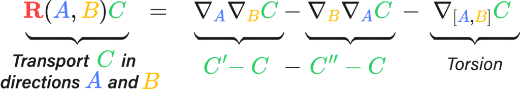
And finally, we comes back to our definition of Riemannian curvature \(R\) we gave in the first section, which uses the difference between left-hand-side and right-hand-side of above condition to model the deviation of this flatness:
$$ R(X,Y)Z=\nabla_X \nabla_Y Z-\nabla_Y \nabla_X Z-\nabla_{[X, Y]} Z $$
In our deformed mesh project, Dr. Nicholas Sharp showed a cool image of discrete parallel transport in his work with Yousuf Soliman and Keenan Crane.
Some “Downsides”
Now, four is good in the sense that it measures deviation from flatness, but it’s still computationally challenging to understand quantitatively. Besides, the Riemannian curvature tensor provides a lot of redundant information: there are a lot of symmetries of components of \(Rm\), namely, the coefficients \(R_{ijkl}\) such that
These symmetries show that knowing some of them allows to get many of the other components. They are good in that taking a glimpse at some of components gets us a full picture, but they are also bad in that these symmetries indicate that there is redundant information encoded in that tensor field.
Preview: The following will be a brief review on some of the common notions of curvature, since understanding of some of them requires a solid base in Tensor algebra.
We seek to use simpler tensor fields to describe curvature. A natural way of doing this is to consider the trace of the Riemannian curvature. We recall from our linear algebra course that the trace of a linear operator \(A\) is the sum of the diagonal elements of its matrix. This concept can be generalized to trace of tensor products, which can be thought of as the sum of diagonal elements of higher-dimensional matrix of tensor products. Ricci curvature \(Rc\) is the trace of \(Rm=R^\flat\) and scalar curvature \(S\) is the trace of \(Rc\).
Thanks to professor Oded Stein, we already learned in our first week SGI tutorial about principal curvature, mean curvature, and Gaussian curvature. Principal curvatures are the largest and smallest plane curve curvatures \(\kappa_1,\kappa_2\) where curves are intersections of a surface and planes aligning with the (outward-pointing) normal vector at point \(p\). This can be generalized to high-dimensional manifolds by observing that the argmin and argmax happen to be eigenvalues of shape operator \(s\) and the fact that \(h(v,v)=\langle sv,v\rangle\) and \(|h(v,v)|\) is the curvature of a curve, where \(h\) is the scalar second fundamental form. Mean curvature is simply the arithmetic mean of eigenvalues of \(s\), namely \(\frac{1}{2}(\kappa_1+\kappa_2)\) in the surface case; Gaussian curvature is the determinant of matrix of \(s\), namely \(\kappa_1\kappa_2\) in the surface case.
It turns out that Gaussian curvature is the bridge between those abstract Riemannian family \(R,Rm, Rc, S\) and above curvatures that are more familiar to us. Gauss was so glad for finding that Gaussian curvature is a local isometry invariant that he named this discovery as Theorema Egregium, Latin for “Remarkable Theorem.” By this theorem, we can talk about Gaussian curvature of a manifold without worrying about where it is embedded. See here for a demo of Gauss map, which is used for his original definition of Gaussian curvature and the proof of the Theorema Egregium (see here for example). This theorem allows us to define the last curvature notion we’ll used: for a given two-dimensional plane \(\Pi\) spanned by vectors \(u,v\in T_pM\), the sectional curvature is defined as the Gaussian curvature of the \(2\)-dimensional submanifold \(S_{\Pi} = \exp_p(\Pi\cap V)\) where \(\exp_p\) is the exponential map and \(V\) is the star-shaped subset of \(T_pM\) for which \(\exp_p\) restricts ot a diffeomorphism.
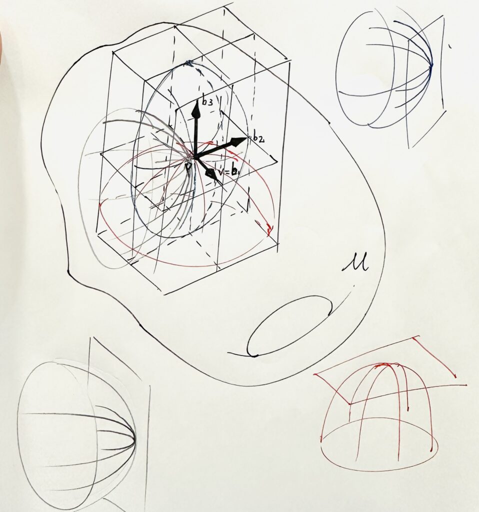
Geometric Interpretation of Ricci and Scalar Curvatures (Proposition 8.32 of Lee’s):
My attempt to visualize sectional curvatures.
Let \((M, g)\) be a Riemannian \(n\)-manifold and \(p \in M\). Then
For every unit vector \(v \in T_p M\), \(Rc_p(v, v)\) is the sum of the sectional curvatures of the 2-planes spanned by \(\left(v, b_2\right), \ldots, \left(v, b_n\right)\), where \(\left(b_1, \ldots, b_n\right)\) is any orthonormal basis for \(T_p M\) with \(b_1 = v\).
The scalar curvature at \(p\) is the sum of all sectional curvatures of the 2-planes spanned by ordered pairs of distinct basis vectors in any orthonormal basis.
General Relativity
Writing: Artur RB Boyago
Introduction: Artur studied physics before studying electrical engineering. Although curvatures of two dimensional objects are much easier to describe, physicists still need higher dimensional analogs to decipher spacetime.
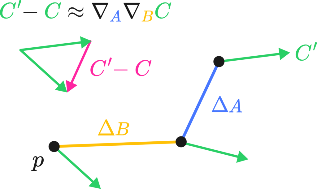
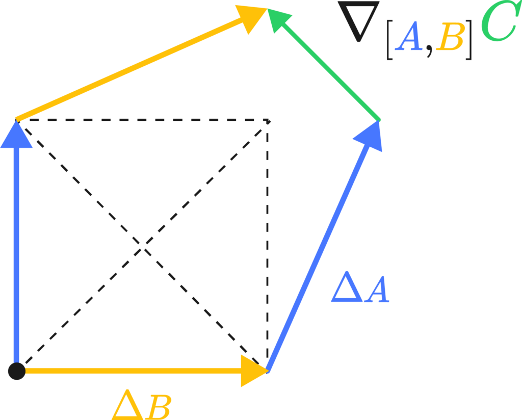
I’d like to give a physicist’s perspective on this whole curvature thing, meaning I’ll flail my hands a lot. The best way I’ve come to understand Riemannian curvature is by the “area/angle deficit” approach. Imagine we had a little bit of a loop made up of two legs, \(\Delta A\) and \( \Delta B\) at a starting point \(p\). Were you to transport a little vector \(C\) down these legs, keeping it as “straight as possible” in curved space. By the end of the two little legs, the vector \( C’ \) would have the same length but a slight rotation in comparison to \(C\). We could, in fact, measure it by taking their difference vector (see the image on the left).
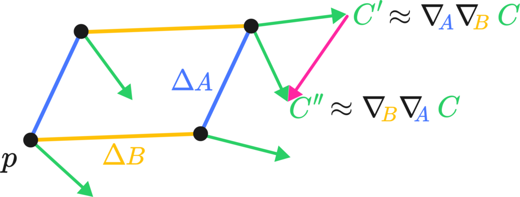
The difference vector is sort of the differential, or the change of the vector along the total path, which we may write down as \( \nabla_A \nabla_B C\), the two covariant derivatives applied to C along \(A\) and \(B\). The critical bit of insight is that changing the order of the transport along \(A\) and \(B\) actually changes the result of said transport. That is, by walking north and then east, and walking east and then north, you end up at the same spot but with a different orientation.
Torsion’s the same deal, but by walking north and then east, and walking east and then north you actually land in a different country.
The Riemann tensor is then actually a fairly simple creature. It has four different instructions in its indices, \(R_{abc}^{\sigma}\), and from the two pictures above we get three of them: Riemann measures the angle deficit or the degree of path-dependance of a region of space. This is the \(R_{abc}\) bit
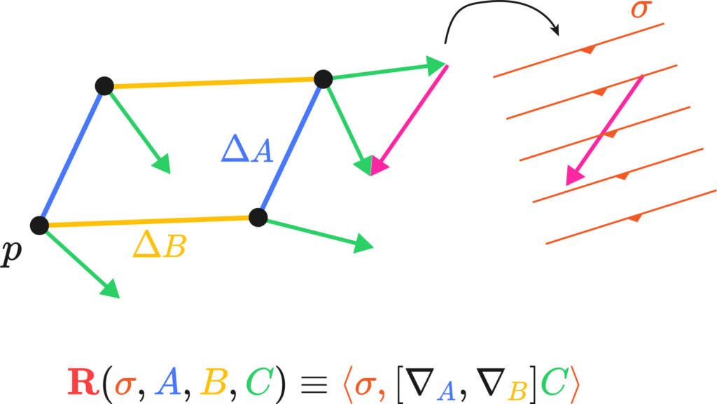
There’s one instruction left. It simply states in which direction we can measure the total difference vector produced by the path by means of a differential form, this closes up our \( R^{\sigma}{abc} \):
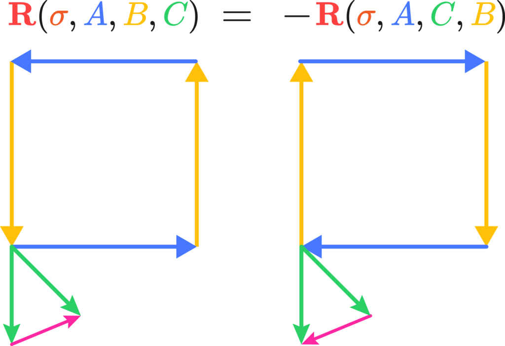
Funny how that works with electrons, they get all confused and get some charge out of frustration. Anyways, the properties of the Riemann tensor can be algebraically understood as these properties of “non-commutative transport” along paths in curved space. For example, the last two indices are naturally anticommutative, since it means the reversal of the direction of travel.
Similarly, it’s quite trivial that by switching the vector being transported and the covector doing the measuring also switches signs: \(R^b_{acd} = -R^a_{bcd}, \; R^a_{bcd} = R^c_{dab}\) The Bianchi Identity is also a statement about what closes and what doesn’t, you can try drawing one that one pretty easily. Now for the general relativity, this is quick; the Einstein tensor is the double dual of the Riemann tensor. It’s hard to see this in tensor calculus, but in geometric algebra it’s rather trivial; the Riemann tensor is a bivector to bivector mapping that produces rotation operators proportional to curvature, the Einstein tensor is a trivector to trivector volume that produces torque curvature operators proportionally to momentum-energy, or momenergy. Torque curvature is an important quantity. The total amount of curvature for the Riemann tensor always vanishes because of some geometry, so if you tried to solve an equation for movement in spacetime you’d be out of luck. But, you can look at the rotational deformation of a volume of space and how much it shrinks proportionally in some section of 3D space. The trick is, this rotational deformation is exactly equal to the content of momentum-energy, or momenergy, of the section. \[\text{(Moment of rotation)} = (e_a\wedge e_b \wedge e_c) \ R^{bc}_{ef} \ (dx_d\wedge dx_e\wedge dx_f) \approx 8\pi (\text{Momentum-energy})\] This is usually written down as\[ \mathbf{G=8\pi T} \]Easy, ay?
If you have an object which you would like to represent as a mesh, what measure do you use to make sure they’re matched nicely?
Suppose you had the ideal, perfectly round implicit sphere \( || \mathbf{x}|| = c\), and you, as a clever geometry processor, wanted to make a discrete version of said sphere employing a polygonal mesh \( \mathbf{M(V,F)}\). The ideal scenario is that by finely tessellating this mesh into a limit of infinite polygons, you’d be able to approach the perfect sphere. However, due to pesky finite memory, you only have so many polygons you can actually add.
The question then becomes, how do you measure how well the perfect and tessellated spheres match? Further, how would you do it for any shape \( f(\mathbf{x}) \)? Is there also a procedure not just for perfect shapes, but also to compare two different meshes? That was the objective of Nicholas Sharp’s research program this week.
The 1D Case
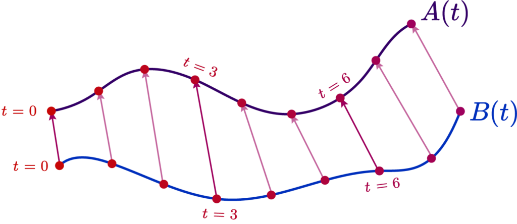
Suppose we had a curve \( A(t):[0,1] \rightarrow \mathbb{R}^n \), and we want to build an approximate polyline curve \( B(t) \). We want to make our discrete points have the nearest look to our original curve \( A(t) \).
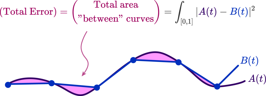
As such, we must choose an error metric measuring how similar the two curves are, and make an algorithm that produces a curve that minimizes this metric. A basic one is simply to measure the total area separating the approximate and real curve, and attempt to minimize it.
The distance between the polyline and the curve \( |A(t) – B(t)| \) is what allows us to produce this error functional, that tells us how much or how little they match. That’s all there is to it. But how do we compute such a distance?
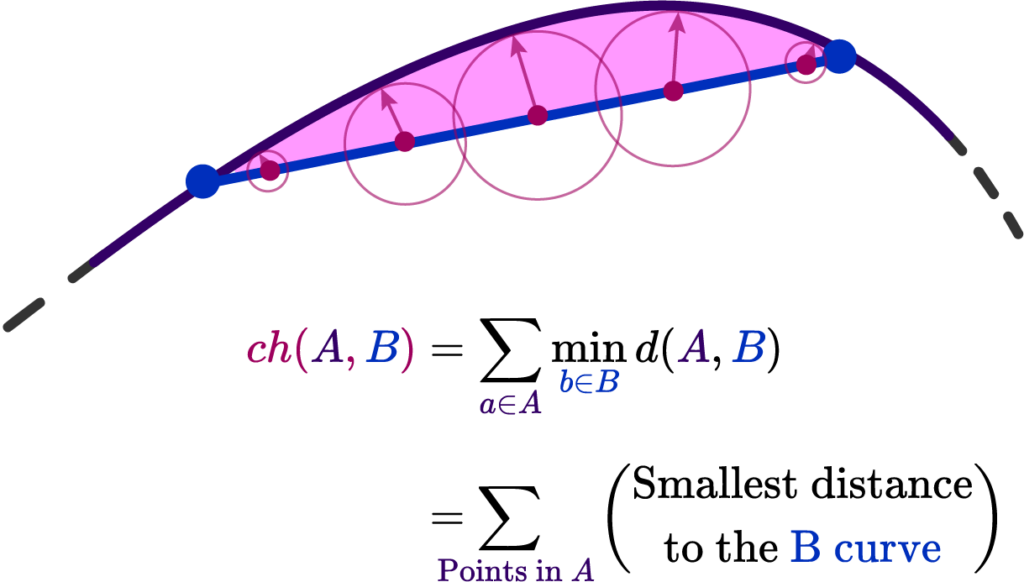
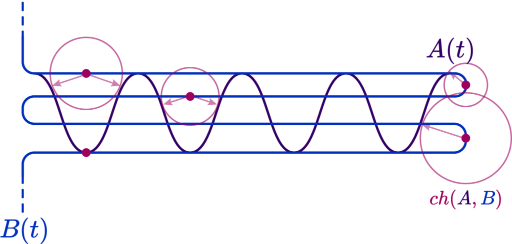
Well, one way is the Chamfer Distance of the two sets of points \( ch(A,B) \). It’s defined as the nearest point distance among the two curves, and all you need to figure it out is to draw little circles along one of the curves. Where the circles touch defines their nearest point!
Here \( d(A,B) \) is just the regular Euclidean distance. Now we would only need to minimize a error functional proportional to \[ \partial E(A,B) = \int_{\gamma} ch(A,B) \sim \sum_{i=0}^n dL \ ch(A, B) = 0 \]
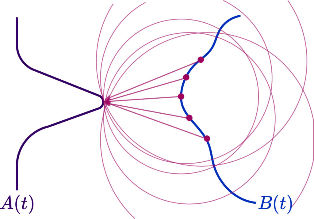
Well simple enough, but there’s a couple of problems. The first one is most evident: a “nearest point query” between curves does not actually contain much geometrical information. A simple counterexample is a spikey curve near a relatively flat curve; the nearest point to a large segment of the curve is a single peak!
We’ll see another soon enough, but this immediately brings into question the validity of an attempted approximation using \( ch(A,B) \). Thankfully mathematicians spent a long time idly making up stuff, so we actually have a wide assortment of possible distance metrics to use!
Different error metrics
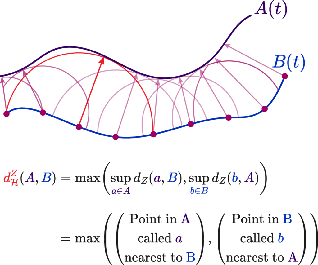
The first alternative metric is the classic Hausdorff Distance, defined as upper bound of the Chamfer distance. Along a curve, always picking the smallest distances, we can select the largest such distance.
Where we to use such a value, the integral error would be akin to the mean error value, rather than the absolute total area. This does not fix our original shape problem, but it does facilitate computation!
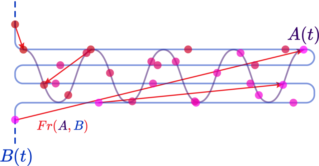
The last contender for our curves is the Fréchet Distance. It is relatively simple: you parametrize two curves \( A \) and \( B \) by some parameter \( t \) such that \(A(\alpha(t)) \) and \( B(\beta(t))\), you can picture it as time; it is always increasing. What we do is say that Fréchet distance \( Fr(A,B) \) is the instantaneous distance between two points “sliding along” the two curves:
We can write this as \[ Fr(A, B) = \inf_{\alpha, \beta} \max_{t\in[0,1]} d(A(\alpha(t)), B(\beta(t))) \]
This provides many benefits at the cost of computation time. The first is that it immediately corrects points from one of our curves “sliding back” as in the peak case, since it must be a completely injective function in the sense one point at some parameter \( t \) must be unique.
The second is that it encodes shape data. The shape information is contained in the relative distribution of the parametrization; for example, if we were to choose \( \alpha(t) \approx \ln t \), we’d produce more “control points” at the tail end of the curve and that’d encode information about its derivatives. The implication being that this information, if associated to the continuity \( (C^n) \) of the curve, could imply details of its curvature and such.
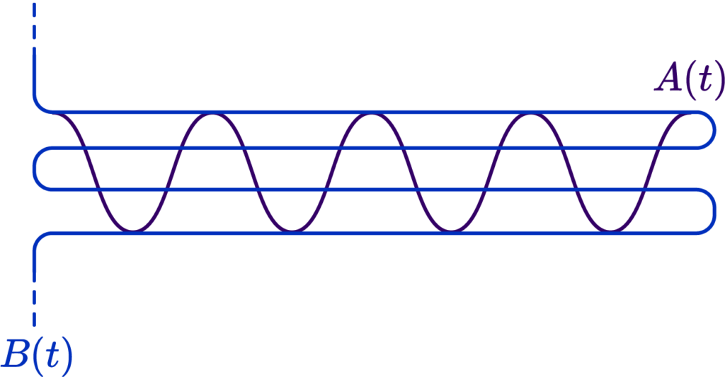
Here is a simple example. Suppose we had two very squiggly curves criss-crossing each other:
Now, were we to choose a Chamfer/Hausdorff distance variant, we would actually get a result indicating a fairly low error, because, due to the criss-cross, we always have a small distance to the nearest point:
However, were we to introduce a parametrization along the two curves that is roughly linear, that is, equidistant along arclenghts of the curve, we could verify that their Fréchet distance is very large, since “same moment in time” points are widely distanced:
Great!
The 2D case
In our experiments with Nicholas, we only got as far as generalizing this method to disk topology, open grid meshes, and using the Chamfer approach to them. We first have a flat grid mesh, and apply a warp function \( \phi(\mathbf{x}) \) that distorts it to some “target” mesh.
def warp_function(uv):

    # input: array of shape (n, 2) uv coordinates. (n,3) input will just ignore the z coordinate

    ret = []
    for i in uv:
        ret.append([i[0], i[1], i[0]*i[1]])

    return np.array(ret)
We used a couple of test mappings, such as a saddle and a plane with a logarithmic singularity.
We then do a Chamfer query to evaluate the absolute error by summing all the distances from the parametric surface to the grid mesh. The 3D Chamfer metric is simply the nearest sphere query to a point in the mesh:
def chamfer_distance(A, B):
    ret = 0
    closest_points = []

    for a in range(A.shape[0]):
        min_distance = float('inf')
        closest_point = None
        for b in range(B.shape[0]):
            distance = np.linalg.norm(A[a] - B[b])
            if distance < min_distance:
                min_distance = distance
                closest_point = b
        ret += min_distance
        closest_points.append((a, A.shape[0]+closest_point))

    closest_points_vertices = np.vstack([A, B])
    closest_points_indices = np.array(closest_points)

    assert closest_points_indices.shape[0] == A.shape[0]
and closest_points_indices.shape[1] == 2
    assert closest_points_vertices.shape[0] == A.shape[0] + B.shape[0] and closest_points_vertices.shape[1] == A.shape[1]

    return ret, closest_points_vertices, closest_points_indices
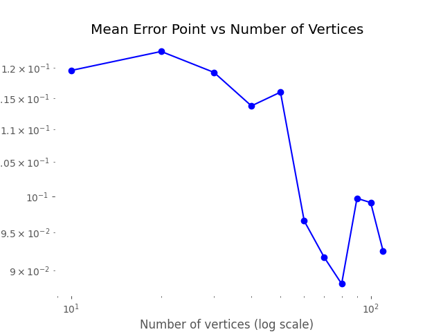
Our main goals were to check if, as the base grid mesh was refined, the error diminished as the approximation increased in resolution, and to see if the relative angle of the grid mesh to the test function significantly altered the error.
The first experiment was validated quite successfully; besides perhaps very pathological cases, the error diminished as we increased the resolution:
And the second one as well, but this will be discussed in a separate blog post.
Application Areas: Chamfer Loss in Action
In machine learning, a loss function is used to measure the difference (i.e. error) between the given input and the neural network’s output. By following this measure, it is possible to have an estimate of how well the neural network models the training data and optimize its weights with respect to this.
For the task of mesh reconstruction, e.g. reconstructing a surface mesh given an input representation such as a point cloud, the loss function aims to measure the difference between the ground truth and predicted mesh. To achieve this, the Chamfer loss (based on the Chamfer distance discussed above) is utilized.
Below, we provide a code snippet for the implementation of Chamfer distance from a widely adopted deep learning library for 3D data, PyTorch3D [1]. The distance can be modified to be used as single or bi-directional (single_directional) and by adopting additional weights.
def chamfer_distance(
    x,
    y,
    x_lengths=None,
    y_lengths=None,
    x_normals=None,
    y_normals=None,
    weights=None,
    batch_reduction: Union[str, None] = "mean",
    point_reduction: Union[str, None] = "mean",
    norm: int = 2,
    single_directional: bool = False,
    abs_cosine: bool = True,

):

    if not ((norm == 1) or (norm == 2)):

        raise ValueError("Support for 1 or 2 norm.")

    x, x_lengths, x_normals = _handle_pointcloud_input(x, x_lengths, x_normals)

    y, y_lengths, y_normals = _handle_pointcloud_input(y, y_lengths, y_normals)

    cham_x, cham_norm_x = _chamfer_distance_single_direction(
        x,
        y,
        x_lengths,
        y_lengths,
        x_normals,
        y_normals,
        weights,
        batch_reduction,
        point_reduction,
        norm,
        abs_cosine,
    )
    if single_directional:
        return cham_x, cham_norm_x

    else:
        cham_y, cham_norm_y = _chamfer_distance_single_direction(

            y,
            x,
            y_lengths,
            x_lengths,
            y_normals,
            x_normals,
            weights,
            batch_reduction,
            point_reduction,
            norm,
            abs_cosine,
        )

        if point_reduction is not None:
            return (
                cham_x + cham_y,
                (cham_norm_x + cham_norm_y) if cham_norm_x is not None else None,
            )
        return (
            (cham_x, cham_y),
            (cham_norm_x, cham_norm_y) if cham_norm_x is not None else None,

        )
When Chamfer is not enough
Depending on the task, the Chamfer loss might not be the best measure to estimate the difference between the surface and reconstructed mesh. This is because in certain cases, the \( k \)-Nearest Neighbor (KNN) step will always be taking the difference between the input point \( \mathbf{y} \) and the closest point \( \hat{\mathbf{y}}\) on the reconstructed mesh, leaving aside the actual point where the measure should be taken into account. This could lead a gap between the input point and the reconstructed mesh to stay untouched during the optimization process. Research for machine learning in geometry proposes to adopt different loss functions to mitigate this problem introduce by the Chamfer loss.
A recent work Point2Mesh [2] addresses this issue by proposing the Beam-Gap Loss. For a point \( \hat{\mathbf{y}}\) sampled from a deformable mesh face, a beam is cast in the direction of the deformable face normal. The beam intersection with the point cloud is the closest point in an \(\epsilon\) cylinder around the beam. Using a cylinder around the beam instead of a single point as in the case of Chamfer distance helps reduce the gap in a certain region between the reconstructed and input mesh.
The beam intersection (or collision) of a point \( \hat{\mathbf{y}}\) is formally given by \( \mathcal{B}(\hat{\mathbf{y}}) = \mathbf{x}\) and the overall beam-gap loss is calculated by:
[1] Ravi, Nikhila, et al. “Accelerating 3d deep learning with pytorch3d.” arXiv preprint arXiv:2007.08501 (2020).
[2] Hanocka, Rana, et al. “Point2mesh: A self-prior for deformable meshes.” SIGGRAPH (2020).
[3] Alt, H., Knauer, C. & Wenk, C. Comparison of Distance Measures for Planar Curves. Algorithmica
[4] Peter Schäfer. Fréchet View – A Tool for Exploring Fréchet Distance Algorithms (Multimedia Exposition).
[5] Aronov, B., Har-Peled, S., Knauer, C., Wang, Y., Wenk, C. (2006). Fréchet Distance for Curves, Revisited. In: Azar, Y., Erlebach, T. (eds) Algorithms
[6] Ainesh Bakshi, Piotr Indyk, Rajesh Jayaram, Sandeep Silwal, and Erik Waingarten. 2024. A near-linear time algorithm for the chamfer distance. Proceedings of the 37th International Conference on Neural Information Processing Systems.
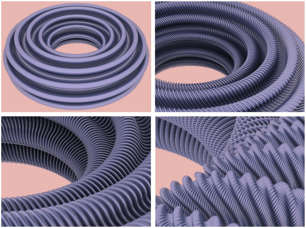
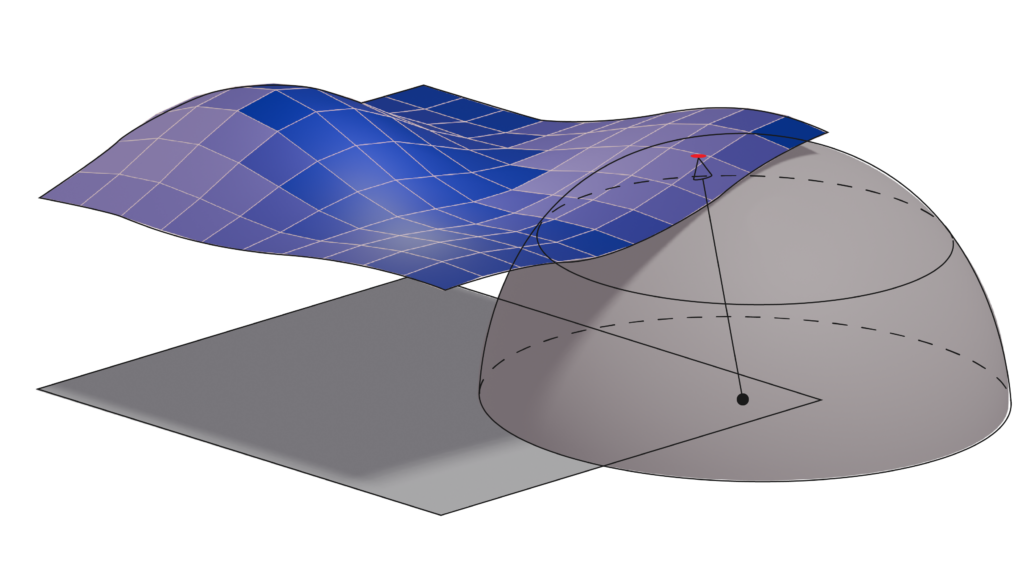
Images: (1) Top left: Wormhole built using Python and Polyscope with its triangle mesh, (2) Top right: Wormhole with no mesh, (3) Bottom left: A concept of a wormhole (credits to: BBC Science Focus, https://www.sciencefocus.com/space/what-is-a-wormhole), (4) A cool accident: an uncomfortable restaurant booth.
During the intense educational week that is SGI’s tutorial week, we stumbled early on, on a challenge: creating our own mesh. A seemingly small exercise to teach us to build a simple mesh, turned for me into much more. I always liked open projects that speak to the creativity of students. Creating our own mesh could be turned into anything and our only limit is our imagination. Although the time was restrictive, I couldn’t but face the challenge. But what would I choose? Fun fact about me: in my studies I started as a physicist before I switched to be an electrical and computer engineer. But my fascination for physics has never faded, so when I thought of a wormhole I knew I had to build it.
From Wikipedia: A wormhole is a hypothetical structure connecting disparate points in spacetime and is based on a special solution of the Einstein field equations. A wormhole can be visualised as a tunnel with two ends at separate points in spacetime.
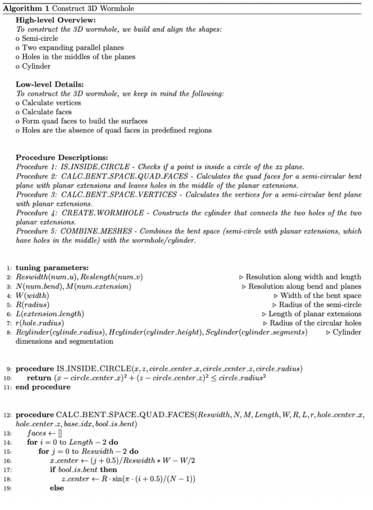
Well, I thought that it would be easier than it really was. It was daunting at first -and during the development I must confess-, but when I started to break the project into steps (first principles thinking), it felt more manageable. Let’s examine the steps on a high level/top-down:
1) build a semi-circle
2) extend its both ends with lines of the same length and parallel to each other
3) make the resulting shape 3D
4) make a hole in the middle of the planes
5) connect the holes via a cylinder
And now let’s explore the bottom-up approach:
1) calculate vertices
2) calculate faces
3) form quad faces to build the surfaces
4) holes are the absence of quad faces in predefined regions
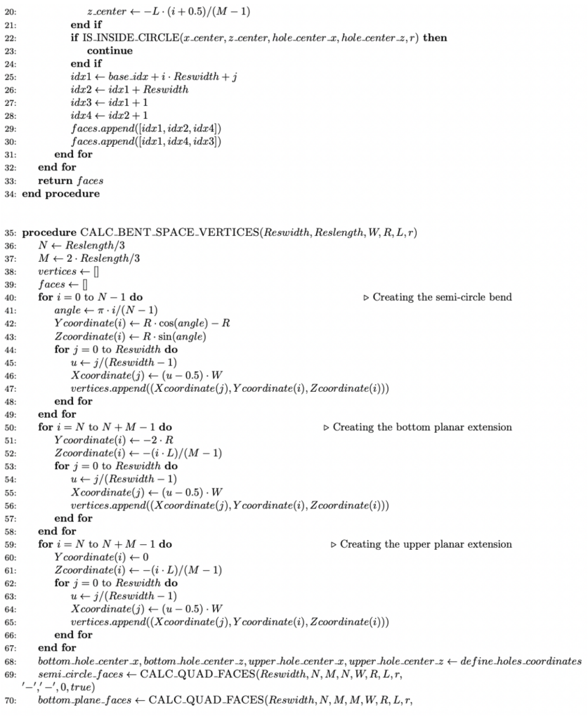
I followed this simple blueprint and the wormhole started to take shape step by step. Instead of giving the details in a never-ending text, I opt to present a high-level algorithm and the GitHub repoof the implementation.
My inspiration for this project? Two-fold; stemming from the very first day of SGI. On one hand, professor Oded Stein encouraged us to be artistic, to create art via Geometry Processing. On the other, Dr. Qingnan Zhou from Adobe shared with us 3 practical tips for us geometry processing newbies:
1) Avoid using background colours, prefer white
2) Use shading
3) Try to become an expert in one of the many tools of Geometry Processing
Well, the third stuck with me, but -of course- I am not close to becoming a master of Python for Geometric Processing and Polyscope, yet. Though, I feel like I made significant strides with this project!
I hope that this work will inspire other students to seek open challenges and creative solutions or even build upon the wormhole, refine it or maybe add a spaceship passing through. Maybe a new SGI tradition? It’s up to you!
P.S. 1: The alignment of the shapes is a little bit overengineered :).
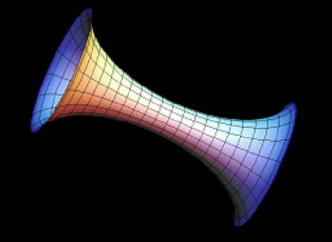
P.S. 2: Unfortunately, it was later in the tutorial week that I was introduced to the 3DXM virtual math museum. Instead of a cylinder, the wormhole should have been a Hyperbolic K=-1 Surface of Revolution, making the shape cleaner:
After Day Two of the first week of SGI Projects (July 16th), Dr. Nicholas Sharp, one of the SGI Tutorial Week lecturers, gave the Fellows a quick glimpse into the powerful open-source program, Blender. Before we jumped into learning how to use Blender, Dr. Sharp highlighted the five key reasons why one might use Blender:
Rendering and Ray tracing
Visual Effects
Mesh modeling and artist content creation *our focus for the tutorial
Physics simulation
Uses node-based and Python-based scripting
Operation: Blender 101
Although one could easily spend hours if not days learning all the techniques and tools of Blender, Dr. Sharp went through how to set up Blender (preferences and how to change the perspective of a mesh) to the basic mesh manipulation and modeling.
Even though we learned many different commands, two of the most essential things to know (at least for me as a novice) were being able to move around the mesh and move the scene. To move around the mesh: use two fingers on your touchpad. To move the scene: hold shift and use two fingers on your touchpad. My favorite trick Dr. Sharp taught was using the spacebar to search for the tool you needed instead of looking around for it.
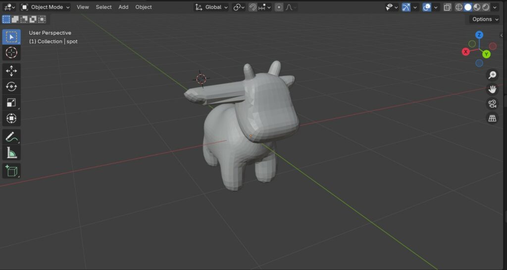
An example of a mesh manipulation we worked on:
By entering edit mode and selecting the faces using the X-ray view, we could select Spot’s ear and stretch it along the X-axis.
Conclusions on Blender
For an open-source program, I was extremely shocked by how powerful and versatile it is, and it makes sense why professionals in the industry could use Blender instead of other paid programs. With his step-by-step explanations, Dr. Sharp was a great teacher and extremely helpful in understanding a program that can be daunting. I’m excited to explore more on how to use Blender and see how I can integrate it into my future endeavors beyond SGI.
By Ashlyn Lee, Mutiraj Laksanawisit, Johan Azambou, and Megan Grosse
Mentored by Professor Yusuf Sahillioglu and Mark Gillespie
The 2D Art Gallery Problem addresses the following question: given an art gallery with a polygonal floor plan, what is the optimal position of security guards to minimize the number of guards necessary to watch over the entirety of the space? This problem has been adapted into the 3D Art Gallery Problem, which aims to minimize the number of guards necessary to guard the entirety of a 3D polygonal mesh. It is this three-dimensional version which our SGI research team explored this past week.
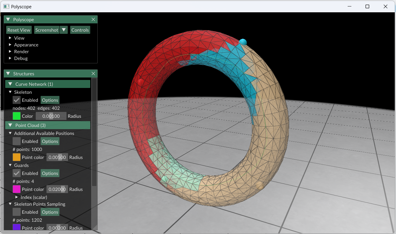
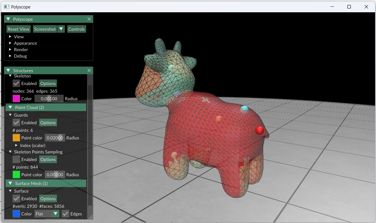
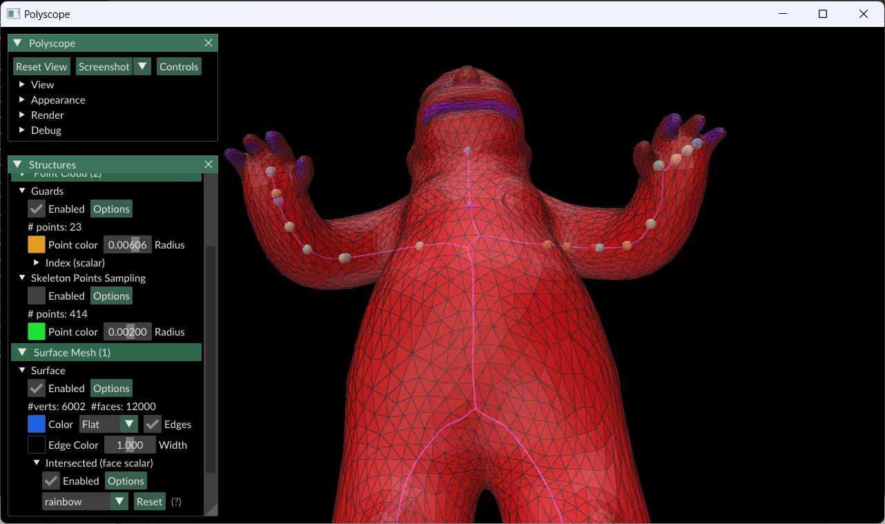
In order to determine what triangular faces a given guarding point g inside of a mesh M could “see,” we defined point p ∈ M as visible to a guarding point g ∈ M if line segment gp lay entirely within M. To implement this definition, we used ray-triangle intersection: starting from each guarding point, our algorithm constructed hypothetical rays passing through the vertices of a small spherical mesh centered on the test point. Then, the first triangle in which each ray intersected was considered “visible.”
Our primary approach to solving the 3D Art Gallery Problem was greedy strategy. Using this method, we can reduce the 3D Art Gallery Problem to a set-covering problem with the set to cover consisting of all faces that make up a given triangle mesh. As part of this method, our algorithm iteratively picked the skeleton point from our sample that could “see” the most faces (as defined by ray-triangle intersection above), and then colored these faces, showing that they were guarded. It then once again picked the point that could cover the most faces and repeated this process with new colors until no faces remained.
However, it turned out that some of our mesh skeletons were not large enough of a sample space to ensure that every triangle face could be guarded. Thus, we implemented a larger sample space of guarding points, also including those outside of the skeleton but within the mesh.
Within this greedy strategy, we attempted both additive and subtractive methods of guarding. The subtractive method involved starting with many guards and removing those with lower guarding capabilities (that were able to see fewer faces). The additive method started with a single guard, placed in the location in which the most faces could be guarded. The additive method proved to be the most effective.
Our results are below, including images of guarded meshes as well as a table comparing skeleton and full-mesh sample points’ numbers of guards and times used:
Model Used
Using only points from the skeleton
(5 attempts)
Adding 1000 more random points
(5 attempts)
No. of Guards
Time Used (seconds)
No. of Guards
Time Used (seconds)
Torus
Min: 7
Max: 8
Avg: 7.2
Min: 6.174
Max: 7.223
Avg: 6.435
Min: 4
Max: 4
Avg: 4
Min: 26.291
Max: 26.882
Avg: 26.494
spot
Unsolvable
Min: 15.660
Max: 16.395
Avg: 16.041
Min: 5
Max: 6
Avg: 5.6
Min: 98.538
Max: 100.516
Avg: 99.479
homer
Unsolvable
Min: 31.210
Max: 31.395
Avg: 31.308
Unsolvable
Min: 232.707
Max: 241.483
Avg: 237.942
baby_doll
Unsolvable
Min: 70.340
Max: 71.245
Avg: 70.840
Unsolvable
Min: 388.229
Max: 400.163
Avg: 395.920
camel
Unsolvable
Min: 91.470
Max: 93.290
Avg: 92.539
Unsolvable
Min: 504.316
Max: 510.746
Avg: 508.053
donkey
Unsolvable
Min: 89.855
Max: 114.415
Avg: 96.008
Unsolvable
Min: 478.854
Max: 515.941
Avg: 488.058
kitten
Min: 4
Max: 5
Avg: 4.2
Min: 41.621
Max: 42.390
Avg: 41.966
Min: 4
Max: 5
Avg: 4.4
Min: 299.202
Max: 311.160
Avg: 302.571
man
Unsolvable
Min: 64.774
Max: 65.863
Avg: 65.200
Unsolvable (⅖)
Min: 15
Max: 15
Avg: 15
Min: 482.487
Max: 502.787
Avg: 494.051
running_pose
Unsolvable
Min: 38.153
Max: 38.761
Avg: 38.391
Unsolvable
Min: 491.180
Max: 508.940
Avg: 500.162
teapot
Min: 10
Max: 11
Avg: 10.2
Min: 39.895
Max: 40.283
Avg: 40.127
Min: 7
Max: 8
Avg: 7.8
Min: 230.414
Max: 235.597
Avg: 233.044
spider
Unsolvable
Min: 151.243
Max: 233.798
Avg: 179.692
Min: 26
Max: 28
Avg: 27
Min: 1734.485
Max: 2156.615
Avg: 1986.744
bunny_fixed
Unsolvable
Min: 32.013
Max: 44.759
Avg: 37.380
Min: 6
Max: 6
Avg: 6
Min: 274.152
Max: 347.479
Avg: 302.596
table
Min: 16
Max: 16
Avg: 16
Min: 358.471
Max: 430.318
Avg: 387.133
Min: 13
Max: 16
Avg: 15.2
Min:1607.658
Max: 1654.312
Avg: 1627.800
lamb
Min: 13
Max: 13
Avg: 13
Min:72.651
Max: 74.011
Avg: 73.480
Min:11
Max: 13
Avg: 11.8
Min: 472.033
Max: 488.215
Avg: 479.064
pig
Min: 12
Max: 13
Avg: 12.4
Min:148.879
Max: 150.889
Avg: 149.670
Min: 15
Max: 17
Avg: 16
Min: 752.750
Max: 789.704
Avg: 766.684
*Note: Unsolvable means that not all of the faces were intersected
Further Research
Given the time restraint, we were unable to explore all of the different approaches and techniques. Firstly, we would ensure all the faces were intersected as it is evident that with our current approach, some of the faces are not getting intersected. This could be applied to the code itself, or the skeleton of the mesh. We could test different approaches of skeletonization to ensure we have the optimal skeleton of the mesh when implementing these approaches. Next, we would have hoped to develop the updated subtractive approach of guarding to compare the results with both additive approaches. We would presume that the results of the runtime for each approach would differ and potentially the location of the guard points as well. Furthermore, we could compare our approaches to those from the literature to determine if we developed a more efficient approach.
Information is attributed to Professor Theodore Kim & Dr. Yoehan Oh
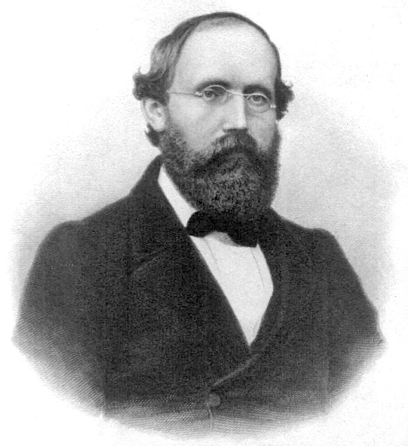
Bui Tuong Phong, 1969
Today, SGI welcomed the incredible Professor Theodore Kim from Yale University, as well as postdoctoral associate Dr. Yoehan Oh, for a Zoom presentation that was just as unique as it was important. While Fellows are spending much of our time focused on the technical side of things, today we took a step back to appreciate the history of a man who deserves more appreciation. With impressive alternation between each of their slide presentations, Professor Kim and Dr. Oh discussed the far-reaching legacy—yet far-too-short life—of Bui Tuong Phong.
Bui Tuong Phong was born in 1942 in Hanoi, Vietnam, but later moved to Saigon in 1954. His history is deeply connected to the Vietnam War—known as the American War in Vietnam. During this time, herbicides with major carcinogens were sprayed in Vietnam, especially in Saigon, while he lived there. It is quite likely that he was exposed.
Bui Tuong eventually left Saigon after being admitted to the Grenoble Institute of Technology in Grenoble, France. He later studied in Paris, and married his wife in 1969. In 1965, the Hart-Cellar Act significantly altered immigration laws in the United States, and he was able to move there. Moreover, the founding of Utah’s CS Division in 1954 provided him with additional support to begin pursuing a PhD at the University of Utah.
After graduation, Bui Tuong taught at Stanford as an adjunct teaching fellow, before his tragically early death in 1975. His cause of death is not known for certain, but the highest possibilities are leukemia, lymphoma, or squamous cell carcinoma. It is quite likely that American war efforts in Vietnam, such as the aforementioned carcinogenic herbicides, may have contributed to his early passing.
Despite all of his efforts, Bui Tuong never got to see how much his work impacted the world. He created the famous Phong shading model and reflection algorithms. Starting with rough shading on a mesh, Bui Tuong interpolated the surface normals to smooth it out, producing a much more realistic and clean mesh. This Phong shading is now the go-to method! Phong reflection added shine in a way that 3D-animated-film-viewers had never seen before—it was satisfyingly realistic. Phong reflection proved to be rather difficult to implement because the position of the viewer’s eye is necessary. Even so, Phong reflection can be seen everywhere now–even in media as popular as Toy Story!
Despite his undeniable contributions to graphics and the entertainment industry, it seems that many are too quick to forget the man behind these contributions. Within mere years of his death, many textbooks and papers even cited his name incorrectly, confusing each of the three parts in his name. After finding such inconsistencies during their research, Professor Kim and Dr. Oh contacted Bui Tuong’s daughter and wife. They confirmed that his family name is Bui Tuong (which can also be correctly written as Bui-Tuong) and his given name is Phong. This raises some interesting questions, like why are Phong shading and reflection named after his given name? Was it Bui Tuong’s own decision, or yet another case of others not taking the time to determine Bui Tuong’s family name vs. given name? Moreover, the top search result photographs allegedly of Bui Tuong are actually not of him at all; rather, they are of an entirely different man who just happens to share Bui Tuong Phong’s given name.
In the profound-yet-saddening words of Dr. Jacinda Tran, “It’s such a cruel irony considering the legacy that [Bui Tuong Phong] left behind: he’s advanced more realistic renderings in the digital realm and yet his own personhood has been so woefully misrepresented.”
Thank you to our guest speakers today for sharing such a moving and important story—and let it be known that Bui Tuong Phong was a man robbed of many years of life, but his incredible legacy lives on.
With week one wrapped up, the SGI 2024 fellows embark on a first adventure into their respective research projects. Today, most of the teams would have already had their first meeting. As we dive deeper into various topics, I wish to write a record of week one– our tutorial week.
Our first day, Monday, 8 July 2024, began with a warm welcome by Dr. Justin Solomon, SGI Director. Without wasting any time, we dove into the introductory material of geometry processing with the guidance of Dr. Oded Stein, who also served as the tutorial week chair. We then had a session on visualizing 3D data with Dr. Qingnan Zhou, a research engineer at Adobe Research.
It is one of the guiding philosophies of SGI that many of the fellows come from various backgrounds. I thought to myself, “not everyone will be at the same skill-level.” To my pleasant surprise, Dr. Stein’s material covered the absolute basics bringing everyone on the call to the same page, or rather presentation slide. The remaining four days followed the same principle, which is something I found admirable.
Our second day, slightly more complicated, was all about parameterization. The introduction was delivered by Richard Liu, a Ph.D. student at the University of Chicago, followed by a lecture on texture maps using PyTorch and texture optimization by Dale Decatur, also a Ph.D. student at UChicago. As a part of their lecture, Richard and Dale also assisted in setting up Jupyter notebooks to complete exercises– it was great help to those new to using such tools.
Since day two was slightly more complicated, there were many great, deep questions about the material. I want to point out the commendable job of the TAs and lecturers themselves on their quick turnaround, succinct answers, and vast resourcefulness. So many papers and articles were exchanged to enhance understanding!
Our third day was a day of realism. Soon-to-be faculty member at Columbia University, Silvia Sellán, covered how the academic community represents 2D- and 3D-shapes. Silvia emphasized the needs of the industry and academic community and offered the pros and cons of each representation. It all came down what a problem needs and what data is available to solve the problem. Silvia also offered a taste of alternate application to common methods and encouraged the 2024 fellows to do the same as they pursue research. The day ended with a guest appearance by Towaki Takikawa, a Ph.D. student from the University of Toronto. Towaki spoke about alternate geometry representations and neural fields with some live demos.
Day four dove deeper into geometry processing algorithms– a special focus on the level-of-detail methods. Which, having understood it, is really intuitive and neat thing to have in our toolbox! This material was taught by Derek Liu, a research scientist at Roblox Inc., and Eris Zhang, a Ph.D. student at Stanford. These talks were the most technical in the tutorial week. I think all the fellows appreciated Derek’s and Eris’s help toward the end of the day to stay back and assist everyone with the exercises.
Our last day was with Dr. Nicholas Sharp, a research scientist at NVIDIA who is also the author of a community-favorite software program, Polyscope. Dr. Sharp focused on what I think is the most important skill in all of programming: debugging. What if we get bad data? How do we deal with data that is beyond what is ideal? Day five was all about code-writing practices and debugging relating to these questions. While this day was technical, Dr. Sharp made it intuitive and easy-to-digest. We also had a complementary session by guest speaker Zachary Ferguson, a postdoc at MIT, on dealing with floating points in collision detection.
Five days of studying all kinds of new things. I, for one, am excited to work on my first project. With such a robust introduction, I feel more confident, as I am sure do others. Good luck to all the fellows, mentors, and volunteers!