Introduction
Early in the very first day of SGI, during professor Oded Stein’s great teaching sprint of the SGI introduction in Geometry Processing, we came across normal vectors. As per his slides: “The normal vector is the unit-length perpendicular vector to a triangle and positively oriented”.
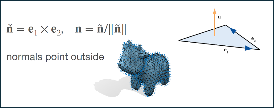
Image 1: The formulas and visualisations of normal vectors in professor Oded Stein’s slides.
Immediately afterwards, we discussed that smooth surfaces have normals at every point, but as we deal with meshes, it is often useful to define per-vertex normals, apart from the well defined per-face normals. So, to approximate normals at vertices, we can average the per-face normals of the adjacent faces. This is the trivial approach. Then, the question that arises is: Going a step further, what could we do? We can introduce weights:

Image 2: Introducing weights to per-vertex normal vector calculation instead of just averaging the per-face normals. (image credits: professor Oded Stein’s slides)
How could we calculate them? The three most common approaches are:
1) The trivial approach: uniform weighting wf = 1 (averaging)
2) area weighting wf = Af
3) angle weighting wf = θf
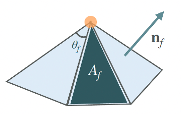
Image 3: The three most common approaches to calculating weights to perform weighted average of the per-face normals for the calculation of per-vertex normals. (image credits: professor Oded Stein’s slides)
During the talk, we briefly discussed the practical side of choosing among the various types of weights and that area weighting is good enough for most applications and, thus, this is the one implemented in gpytoolbox, a Geometry Processing python package that professor Oded Stein has significantly contributed to its development. Then, he gave us an open challenge: whoever was up for the challenge could implement the angle-weighted per-vertex normal calculation and contribute it to gpytoolbox! I was intrigued and below I give an overview of my implementation of the per_vertex_normals(V, F, weights=’area’, correct_invalid_normals=True) function.
Implementation Overview
First, I implemented an auxiliary function called compute_angles(V,F). This function calculates the angles of each face using the dot product between vectors formed by the vertices of each triangle. The angles are then calculated using the arccosine of the dot product cosine result. The steps are:
- For each triangle, the vertices A, B, and C are extracted.
- Vectors representing the edges of each triangle are calculated:
AB=B−A
AC=C−A
BC=C−B
CA=A−C
BA=A−B
CB=B−C
- The cosine of each angle is computed using the dot product:
cos(α) = (AB AC)/(|AB| |AC|)
cos(β) = (BC BA)/(|BC| |BA|)
cos(γ) = (CA CB)/(|CA| |CB|)
- At this point, the numerical issues that can come up in geometry processing applications that we discussed on day 5 with Dr. Nicholas Sharp came to mind. What if the values of arccos(angle) exceed the values 1 or -1? To avoid potential numerical problems I clipped the results to be between -1 and 1:
α=arccos(clip(cos(α),−1,1))
β=arccos(clip(cos(β),−1,1))
γ=arccos(clip(cos(γ),−1,1))
Having compute_angles, now we can explore the per_vertex_normals function. It is modified to get an argument to select weights among the options: “uniform”, “angle”, “area” and applies the selected weight averaging of the per-face normals, to calculate the per-vertex normals:
def per_vertex_normals(V, F, weights=’area’, correct_invalid_normals=True):
- Make sure that the V and F data structures are of types float64 and int32 respectively, to make our function compatible with any given input
- Calculate the per face normals using gpytoolbox
- If the selected weight is “area”, then use the already implemented function.
- If the selected weight is “angle”:
- Compute angles using the compute_angles auxiliary function
- Weigh the face normals by the angles at each vertex (weighted normals)
- Calculate the norms of the weighted normals
(A small parenthesis: The initial implementation of the function implemented the 2 following steps:
- Include another check for potential numerical issues, replacing very small values of norms that may have been rounded to 0, with a very small number, using NumPy (np.finfo(float).eps)
- Normalize the vertex normals: N = weighted_normals / norms
Can you guess the problem of this approach?*)
6. Identify indices with problematic norms (NaN, inf, negative, zero)
7. Identify the rest of the indices (of valid norms)
8. Normalize valid normals
9. If correct_invalid_normals == True
- Build KDTree using only valid vertices
- For every problematic index:
- Find the nearest valid normal in the KDTree
- Assign the nearest valid normal to the current problematic normal
- Else assign a default normal ([1, 0, 0]) (in the extreme case no valid norms are calculated)
- Normalise the replaced problematic normals
10. Else ignore the problematic normals and just output the valid normalised weighted normals
*Spoiler alert: The problem of the approach was that -in extreme cases- it can happen that the result of the normalization procedure does not have unit norm. The final steps that follow ensure that the per-vertex normals that this function outputs always have norm 1.
Testing
A crucial stage of developing any type of software is testing it. In this section, I provide the visualised results of the angle-weighted per-vertex normal calculations for base and edge cases, as well as everyone’s favourite shape: spot the cow:
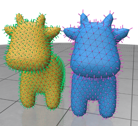
Image 4: Let’s start with spot the cow, who we all love. On the left, we have the per-face normals calculated via gpytoolbox and on the right, we have the angle-weighted per-vertex normals, calculated as analysed in the previous section.

Image 5: The base case of a simple triangle.

Image 6: The base case of an inverted triangle (vertices ordered in a clockwise direction)
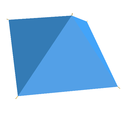
Image 7: The base case of a simple pyramid with a base.

Image 8: The base case of disconnected triangles.
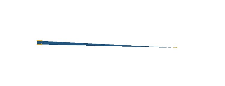
Image 9: The edge case of having a very thin triangle.
Finally, for the cases of a degenerate triangle and repeated vertex coordinates nothing is visualised. The edge cases of having very large or small coordinates have also been tested successfully (coordinates of magnitude 1e8 and 1e-12, respectively).
Having a verified visual inspection is -of course- not enough. The calculations need to be compared to ground truth data in the context of unit tests. To this end, I calculated the ground truth data via the sibling of gpytoolbox: gptoolbox, which is the respective Geometry Processing package but in MATLAB! The shape used to assert the correctness of our per_vertex_normals function, was the famous armadillo. Tests passed for both angle and uniform weights, hurray!
Final Notes
Developing the weighted per-vertex normal function and contributing slightly to such a powerful python library as gpytoolbox, was a cool and humbling experience. Hope the pull request results into a merge! I want to thank professor Oded Stein for the encouragement to take up on the task, as well as reviewing it along with the soon-to-be professor Silvia Sellán!