
This post serves as a tutorial for using RXMesh.
RXMesh is a framework for processing triangle mesh on the GPU. It allows developers to easily use the GPU’s massive parallelism to perform common geometry processing tasks.
This tutorial will cover the following topics:
- Setting up RXMesh
- RXMesh basic workflow
- Writing kernels for queries
- Example: Visualizing face normals
Setting up RXMesh
For the sake of this tutorial, you can set up a fork of RXMesh and then create your own small section to implement your own tutorial examples in the fork.
Go to https://github.com/owensgroup/RXMesh and fork the repository. You can create your own directory with a simple CUDA script to start using RXMesh. To do so, go to https://github.com/owensgroup/RXMesh/blob/main/apps/CMakeLists.txt in your fork and add a line:
add_subdirectory(introduction)In the apps directory on your local fork, create a folder called “introduction”. There should be two files in this folder.
- A .cu file to run the code. You can call this introduction.cu. To start, it can have the following contents:
#include "rxmesh/query.cuh"
#include "rxmesh/rxmesh_static.h"

#include "rxmesh/matrix/sparse_matrix.cuh"

using namespace rxmesh;

int main(int argc, char** argv)
{
    Log::init();

    const uint32_t device_id = 0;
    cuda_query(device_id);

    RXMeshStatic rx(STRINGIFY(INPUT_DIR) "sphere3.obj");

#if USE_POLYSCOPE
    polyscope::show();
#endif
}
2. A CMake file called CMakeLists.txt. It must have the following contents:
add_executable(introduction)

set(SOURCE_LIST
    introduction.cu
)

target_sources(introduction
    PRIVATE
    ${SOURCE_LIST}
)

set_target_properties(introduction PROPERTIES FOLDER "apps")

set_property(TARGET ARAP PROPERTY CUDA_SEPARABLE_COMPILATION ON)

source_group(TREE ${CMAKE_CURRENT_LIST_DIR} PREFIX "introduction" FILES ${SOURCE_LIST})

target_link_libraries(introduction
    PRIVATE RXMesh
)

#gtest_discover_tests( introduction )
Once you have done the above steps, building the project with CMake is simple. Refer to the README in https://github.com/owensgroup/RXMesh to know the requirements and steps to build the project for your device.
Once the project has been set up, we can begin to test and run our introduction.cu file. If you were to run it, you should get an output of a 3D sphere.
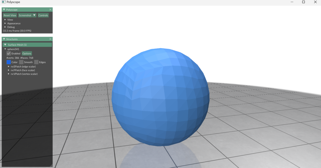
This means the project set up has been successful, we can now begin learning RXMesh.
RXMesh basic workflow
RXMesh provides custom data structures and functions to handle various low-level computational tasks that would otherwise require low-level implementation. Let’s explore the fundamentals of how this workflow operates.
To start, look at this piece of code.
int main(int argc, char** argv)
{
Log::init();
const uint32_t device_id = 0;
rxmesh::cuda_query(device_id);
rxmesh::RXMeshStatic rx(STRINGIFY(INPUT_DIR) "dragon.obj");
auto polyscope_mesh = rx.get_polyscope_mesh();
auto vertex_pos = *rx.get_input_vertex_coordinates();
auto vertex_color = *rx.add_vertex_attribute<float>("vColor", 3);
rx.for_each_vertex(rxmesh::DEVICE,
[vertex_color, vertex_pos] __device__(const rxmesh::VertexHandle vh)
{
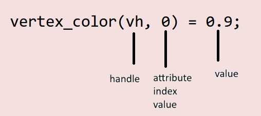
vertex_color(vh, 0) = 0.9;
vertex_color(vh, 1) = vertex_pos(vh, 1);
vertex_color(vh, 2) = 0.9;
});
vertex_color.move(rxmesh::DEVICE, rxmesh::HOST);
polyscope_mesh->addVertexColorQuantity("vColor", vertex_color);
polyscope::show();
return 0;
}The above is a slightly simplified version of what a for_each computation program would look like using RXMesh. for_each involves accessing every mesh element of a specific type (vertex, edge, or face) and performing some process on/with it.
In the code example above, the computation adjusts the green component of the vertex’s color based on the vertex’s Y coordinate in 3D space.
But how do we comprehend this code? We will look at it line by line:
rxmesh::RXMeshStatic rx(STRINGIFY(INPUT_DIR) "dragon.obj");The above line declares the RXMeshStatic object. Static here stands for a static mesh (one whose connectivity remains constant for the duration of the program’s runtime). Using the RXMesh’s Input directory, we can use some meshes that come with it. In this case, we pass in the dragon.obj file, which holds the mesh data for a dragon.
auto polyscope_mesh = rx.get_polyscope_mesh();This line returns the data needed for Polyscope to display the mesh along with any attribute content we add to it for visualization.
auto vertex_pos = *rx.get_input_vertex_coordinates();This line is a special function that directly gives us the coordinates of the input mesh.
auto vertex_color = *rx.add_vertex_attribute<float>("vColor", 3);This line gives vertex attributes called “vColor”. Attributes are simply data that lives on top of vertices, edges, or faces. To learn more about how to handle attributes in RXMesh, check out this. In this case, we associate three float-point numbers to each vertex in the mesh.
rx.for_each_vertex(rxmesh::DEVICE,
    [vertex_color, vertex_pos] __device__(const rxmesh::VertexHandle vh)
    {
            vertex_color(vh, 0) = 0.9;
            vertex_color(vh, 1) = vertex_pos(vh, 1);
            vertex_color(vh, 2) = 0.9;
    });
The above lines represent a lambda function that is utilized by the for_each computation. In this case, for_each_vertex accesses each of the vertices of the mesh associated with our dragon. We pass in the arguments:
rxmesh::DEVICE– to let RXMesh know this is happening on the device i.e., the GPU.[vertex_color, vertex_pos]– represents the data we are passing to the function.(const rxmesh::VertexHandle vh)– is the handle that is used in any RXMesh computation. A handle allows us to access data associated to individual geometric elements. In this case, we have a handle that allows us to access each vertex in the mesh.
What do these lines mean?
            vertex_color(vh, 0) = 0.9;
            vertex_color(vh, 1) = vertex_pos(vh, 1);
            vertex_color(vh, 2) = 0.9;
These 3 lines bring together a lot of the declarations made earlier. Through the kernel, we are accessing the attribute data we defined before. Since we need to know which vertex we are accessing its color, we pass in vh as the first argument. Since a vertex has three components (standing for RGB), we also need to pass which index in the attribute’s vector (you can think of it as a 1D array too) we are accessing. Hence vertex_color(vh, 0) = 0.9; which stands for “in the vertex color associated with the handle vh (which for the kernel represents a specific vertex on the mesh), the value of the first component is 0.9”. Note that this “first component” represents red for us.
What about vertex_color(vh, 1) = vertex_pos(vh, 1)? This line, similar to the previous one, is accessing the second component associated with the color, in the vertex the handle is associated with.
But what is on the right-hand side? We are accessing vertex_pos (our coordinates of each vertex in the mesh) and we are accessing it the same way we access our color. In this case, the line is telling us that we are accessing the 2nd positional coordinate (y coordinate) associated with our vertex (that our handle gives to the kernel).
vertex_color.move(rxmesh::DEVICE, rxmesh::HOST);This line moves the attribute data from the GPU to the CPU.
polyscope_mesh->addVertexColorQuantity("vColor", vertex_color);This line uses Polyscope to add a “quantity” to Polyscope’s visualization of the mesh. In this case, when we add the VertexColorQuantity and pass vertex_color, Polyscope will now visualize the per-vertex color information we calculated in the lambda function.
polyscope::show();We finally render the entire mesh with our added quantities using the show() function from Polyscope.
Throughout this basic workflow, you may have noticed it works similarly to any other program where we receive some input data, perform some processing, and then render/output it in some form.
More specifically, we use RXMesh to read that data, set up our attributes, and then pass that into a kernel to perform some processing. Once we move that data from the device to the host, we can either perform further processing or render it using Polyscope.
It is important to look at the kernel as computing per geometric element. This means we only need to think of computation on a single mesh element of a certain type (i.e., vertex, edge, or face) since RXMesh then takes this computation and runs it in parallel on all mesh elements of that type.
Writing kernels for queries
While our basic workflow covers how to perform for_each operation using the GPU, we may often require geometric connectivity information for different geometry processing tasks. To do that, RXMesh implements various query operations. To understand the different types of queries, check out this part of the README.
We can say there are two parts to run a query.
The first part consists of creating the launchbox for the query, which defines the threads and (shared) memory allocated for the process along with calling the function from the host to run on the device.
The second part consists of actually defining what the kernel looks like.
We will look at these one by one.
Here’s an example of how a launchbox is created and used for a process where we want to find all the vertex normals:
// Vertex Normal
auto vertex_normals = rx.add_vertex_attribute("vNormals", 3);
constexpr uint32_t CUDABlockSize = 256;

rxmesh::LaunchBox<CUDABlockSize> launch_box;

rx.prepare_launch_box(
  {rxmesh::Op::FV},
  launch_box,
  (void*)compute_vertex_normal<float,CUDABlockSize>);

compute_vertex_normal<float, CUDABlockSize>
<<<launch_box.blocks,
   launch_box.num_threads,
   launch_box.smem_bytes_dyn>>>
(rx.get_context(), vertex_pos, *vertex_normals);

vertex_normals->move(rxmesh::DEVICE, rxmesh::HOST);
Notice how, in replacing the for_each part of our basic workflow, we instead declare the launchbox and call our function compute_vertex_normal (which we will look at next) from our main function.
We must also define the kernel which will run on the device.
template <typename T, uint32_t blockThreads>
__global__ static void compute_vertex_normal(const rxmesh::Context      context,
rxmesh::VertexAttribute<T> coords,
rxmesh::VertexAttribute<T> normals)
{


    auto vn_lambda = [&](FaceHandle face_id, VertexIterator& fv){
        // get the face's three vertices coordinates
        glm::fvec3 c0(coords(fv[0], 0), coords(fv[0], 1), coords(fv[0], 2));
        glm::fvec3 c1(coords(fv[1], 0), coords(fv[1], 1), coords(fv[1], 2));
        glm::fvec3 c2(coords(fv[2], 0), coords(fv[2], 1), coords(fv[2], 2));

        // compute the face normal
        glm::fvec3 n = cross(c1 - c0, c2 - c0);

        // the three edges length
        glm::fvec3 l(glm::distance2(c0, c1),
                     glm::distance2(c1, c2),
                     glm::distance2(c2, c0));

        // add the face's normal to its vertices
        for (uint32_t v = 0; v < 3; ++v) {
// for every vertex in this face
            for (uint32_t i = 0; i < 3; ++i) {
// for the vertex 3 coordinates
                atomicAdd(&normals(fv[v], i), n[i] / (l[v] + l[(v + 2) % 3]));
            }
        }
    };

    auto block = cooperative_groups::this_thread_block();

    Query<blockThreads> query(context);
    ShmemAllocator      shrd_alloc;
    query.dispatch<Op::FV>(block, shrd_alloc, vn_lambda);
}
A few things to note about our kernel
- We pass in a few arguments to our kernel.
- We pass the
contextwhich allows RXMesh to access the data structures on the device. - We pass in the coordinates of each vertex as a
VertexAttribute - We pass in the normals of each vertex as an attribute. Here, we accumulate the face’s normal on its three vertices.
- We pass the
- The function that performs the processing is a lambda function. It takes in the handles and iterators as arguments. The type of the argument will depend on what type of query is used. In this case, since it is an FV query, we have access to the current face(
face_id) the thread is acting on as well as the vertices of that face usingfv. - Notice how within our lambda function, we do the same as before with our
for_eachoperation, i.e., accessing the data we need using the attribute handle and processing it for some output for our attribute. - Outside our lambda function, notice how we need to set some things up with regards to memory and the type of query. After that, we call the lambda function to make it run using
query.dispatch
Visualizing face normals
Now that we’ve learnt all the pieces required to do some interesting calculations using RXMesh, let’s try a new one out.
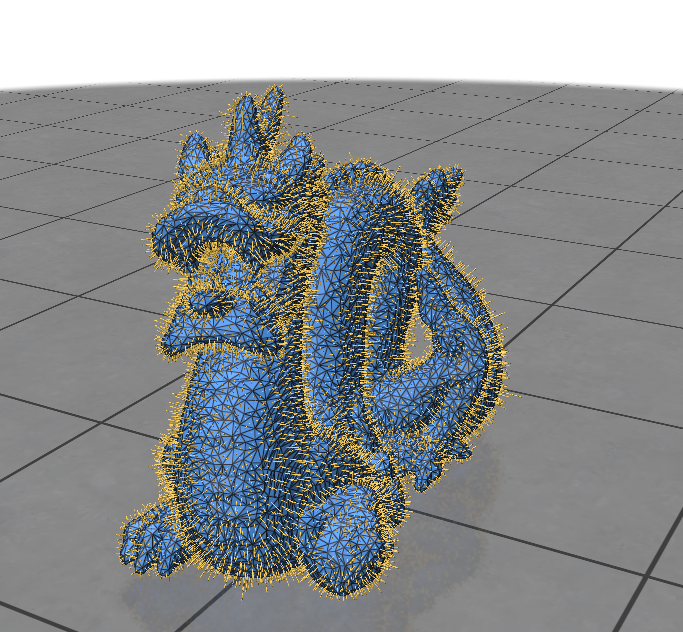
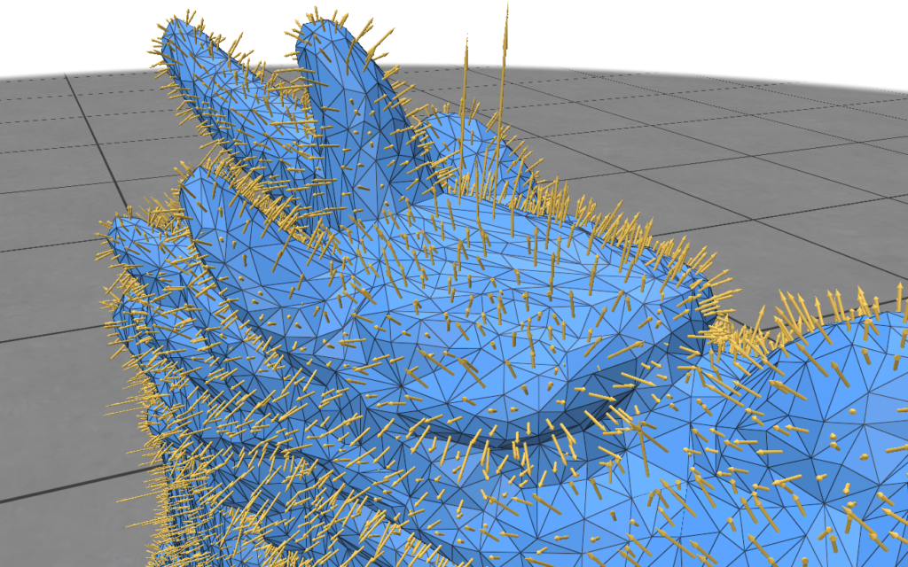
Try to visualize the face normals of a given mesh. This would mean obtaining an output like this for the dragon mesh given in the repository:
Here’s how to calculate the face normals of a mesh:
- Take a vertex. Calculate two vectors that are formed by subtracting the selected vertex from the other two vertices.
- Take the cross product of the two vectors.
- The vector obtained from the cross product is the normal of the face.
Now try to perform the calculation above. We can do this for each face using the vertices it is connected to.
All the information above should give you the ability to implement this yourself. If required, the solution is given below.
The kernel that runs on the device:
template <typename T, uint32_t blockThreads>
global static void compute_face_normal(
const rxmesh::Context context,
rxmesh::VertexAttribute coords, // input
rxmesh::FaceAttribute normals) // output
{
auto vn_lambda = [&](FaceHandle face_id, VertexIterator& fv) {
    // get the face's three vertices coordinates

    glm::fvec3 c0(coords(fv[0], 0), coords(fv[0], 1), coords(fv[0], 2));
    glm::fvec3 c1(coords(fv[1], 0), coords(fv[1], 1), coords(fv[1], 2));
    glm::fvec3 c2(coords(fv[2], 0), coords(fv[2], 1), coords(fv[2], 2));

    // compute the face normal
    glm::fvec3 n = cross(c1 - c0, c2 - c0);
    normals(face_id, 0) = n[0];
    normals(face_id, 1) = n[1];
    normals(face_id, 2) = n[2];
};

auto block = cooperative_groups::this_thread_block();
Query<blockThreads> query(context);
ShmemAllocator shrd_alloc;
query.dispatch<Op::FV>(block, shrd_alloc, vn_lambda);

}
The function call from main on HOST:
int main(int argc, char** argv)
{
    Log::init();

    const uint32_t device_id = 0;
    cuda_query(device_id);

    rxmesh::RXMeshStatic rx(STRINGIFY(INPUT_DIR) "sphere3.obj");

    auto vertex_pos = *rx.get_input_vertex_coordinates();
    auto face_normals = rx.add_face_attribute<float>("fNorm", 3);

    constexpr uint32_t CUDABlockSize = 256;
    LaunchBox<CUDABlockSize> launch_box;

    compute_face_normal<float, CUDABlockSize>
    <<<launch_box.blocks,
    launch_box.num_threads,
    launch_box.smem_bytes_dyn>>>
    (rx.get_context(), vertex_pos, *face_normals);

    face_normals->move(DEVICE, HOST);

    rx.get_polyscope_mesh()->addFaceVectorQuantity("fNorm", *face_normals);

#if USE_POLYSCOPE
    polyscope::show();
#endif
}
As an extra example, try the following:
- Color a vertex depending on how many vertices it is connected to.
- Test the above on different meshes and see the results. You can access different kinds of mesh files from the “Input” folder in the RXMesh repo and add your own meshes if you’d like.
By the end of this, you should be able to do the following:
- Know how to create new subdirectories in the RXMesh Fork
- Know how to create your own
for_eachcomputations on the mesh - Know how to create your own queries
- Be able to perform some basic geometric analyses’ using RXMesh queries
References
More information can be found in RXMesh GitHub Repository.
This blog was written by Sachin Kishan during the SGI 2024 Fellowship as one of the outcomes of a two week project under the mentorship of Ahmed Mahmoud and support of Supriya Gadi Patil as teaching assistant.