Categories
Research

Arc-Length Splines

Introduction

A spline is a function that usually represents a piecewise polynomial. Splines have a variety of applications, from being used to visualize a curve to representing motion in animation, to model a surface, or for artistic visualizations. 

Our project on Arc Length Splines aimed to satisfy a new necessity in spline formulation- an analytically computable arc length. We aim to allow users to output the arc length and further constrain the spline using the arc length. Further, we want to ensure some amount of continuity on the spline.

Background

Continuity

In the context of splines, continuity can be defined as having no sudden change in value across the spline function. There are two kinds of continuity discussed here, namely parametric (C) and geometric (G) continuity. 

There are different levels of continuity dubbed C1 continuity, C2 continuity, and so on until Cn continuity. (The same applies to G as well)

A Ci continuous spline is defined as one where for a function f(t) that defines the spline, f i (t) is continuous for all points t, where i represents the order of the derivative. This is usually true for each curve that is in the spline. The points of interest where continuity may not occur are at the points where two curves meet, called the joints. To verify if there is continuity at the joints, we can use the following method: 

Assume we have two curves A and B where the endpoint of A is connected to the starting point of B. These curves are parameterized on the domain [0,1].

A and B form a Ci continuous spline if 

Ai (1) = Bi (0)

This can be used to verify any spline made of an arbitrary number of curves, given that for every two consecutive curves connected at a joint, they satisfy the above condition. 

Any Ci spline is also C0, C1 … Ci-2, Ci-1continuous.

Gi continuity is based on the “geometric” smoothness of the curve. Where G1 is the continuity at the tangents along the spline. G2 continuity refers to the continuty of the curvature along the spline. 

Continuity plays an important role in how a spline’s application may behave. For example, if a spline is acting as a path for an object moving along it, if the spline is not C1 continuous (meaning each consecutive curve has an endpoint that meets at the joint of the spline but with discontinuities for the first differential), the spline may not be useful. This is because objects would likely move at different speeds along different curves(or increase and decrease in speed at the joints.) This is what makes continuity a desirable property in spline applications. 

Approximating vs interpolating control points

Splines can be changed based on their control points. Splines that go through the entire set of control points are called interpolating splines (since they interpolate between the entire given set of control points). In an approximating spline, the spline approximates the polyline made by the control points into a smooth curve. 

Local and Global control

Based on the constraints on the spline formulation, the control points have influence over certain parts of the spline. In cases where a control point only effects the curve at which it acts as a joint (or is the point that directly decides how two curve segments are to be formed), the spline is said to have control points with local control. (Local being the curves before and after the control point at a joint). 

In some cases, constraints may influence larger parts of the spline beyond local curves, this is referred to as global control. 

It is usually desirable to have local control for applications like spline drawing, where we want to create a curve of a certain visual form without largely impacting the rest of the spline it is a part of.

Arc Length

Arc length is the distance along the curve given two points on the curve. For any arbitrary curves, arc length can be integrated between two points. For special curves such as circles or parabolas, there is an analytically computed arc length. Our choice of curve and interpolation schemes to explore were driven by where we could analytically calculate arc length for a curve. This also influenced other considerations of our spline.

Past Work

Most of our inspiration came from the paper “A Class of C^2 Interpolating Splines” by Cem Yuksel(2020). Yuksel was able to classify four different types of splines that maintained C^2 continuity and interpolation. These were splines using the Bézier interpolation function, circular interpolation function, elliptical interpolation function, and hybrid (circular-elliptical) interpolation function. Yuksel(2020) used a combination of the base curve and a blending function to maintain continuity. 

The use of a blending function is excellent for ensuring continuity between different kinds of curves. However, our goal is to have an exact arc length. The function Yuksel(2020) uses was a second order trigonometric function. Thus, there was no closed formula for the arc-length of for the blending function.

Our work

After initial review of past literature- we compiled a set of curves in which an analytical solution for arc length exists. We dived deeper into curves which have closed formula arc length. The main curves of this family are circles, parabolas, catenoids, and the logarithmic spiral. We then focussed on creating splines out of this initial set of curves. Through this process, we recognised that circular curves may be the best option, not only because their arc length is easy to calculate, but presented properties to create a locally controllable spline with C1 continuity.

A spline is formed when we connect an endpoint of two curves to each other. To formulate a circular spline, there are different ways to connect them. One option was to just draw line segments between two arcs. The problem is that this may not always be continuous if further constraints are not provided.

Another way to connect two circular arcs is to use the Dubins Path. Dubins Paths are usually used in robotics or car path planning. Since they are used to find the shortest path between any two curves which have constraints on curvature, they work perfectly to find a connecting path between two circular arcs.

Dubin’s path between two circular arcs, which turns out to be a line segment. Source: Salix Alba [2]

If a line segment between two curves is not a line segment, Dubin’s path instead form it’s own curve to draw between the two. These are known as CCC paths (where C stands for curve).

Dubin’s path between two circular arcs, which turns out to be another circular arc. Source: Salix Alba [3]

This ensures we no longer constrain user outcome and provide additional output for a user to adjust visually. The arc length of a Dubins path can also be computed analytically. This is because in all possible cases of a Dubins path, the path will either be a line segment or another circular arc. This allows for the analytical calculation of arc length across the entire spline while also ensuring C1 continuity. This fits with our requirements for an arc-length computable spline retaining at least a C1 continuity property.

We then worked on implementing the idea above: a set of circular arcs whose spline is formed with the dubins path connecting them. 

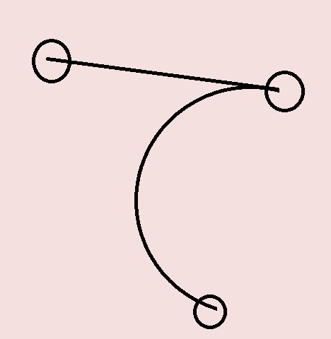
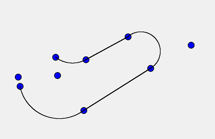
To implement circular arcs, we used two points and a tangent from one of them to determine a circular arc. This would equate to 3 points used per arc. Using a set of 6 points (which form 2 circular arcs), we then create a path between them. 

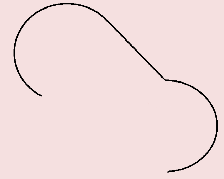
Our current implementation allows for the creation of circular arcs with straight paths formed between them.

Our implementation in python. Each arc is made of three points and is connected by a line segment

Future work 

Our current implementation is limited, we intend to improve it in the following ways:

  1. Ensure a Dubins path for all cases of circular arcs
  2. Create arc length constraints as well as outputs for users to view and edit
  3. Better interface to clearly demarcate between different curves, tangent points and circular arc points.
  4. Implementing higher order continuity while ensuring lesser constraints on spline editing.

References

[1] Cem Yuksel. 2020. A Class of C2 Interpolating Splines. ACM Trans. Graph. 39, 5, Article 160 (October 2020), 14 pages. https://doi.org/10.1145/3400301

[2] Salix Alba (2016, 6 February) Dubins3.svg https://upload.wikimedia.org/wikipedia/commons/e/e7/Dubins3.svg

[3] Salix Alba (2016, 6 February) Dubins2.svg https://upload.wikimedia.org/wikipedia/commons/e/e7/Dubins2.svg

[4] Freya Holmér. (2022, December 7). The continuity of Splines [Video]. YouTube. https://www.youtube.com/watch?v=jvPPXbo87ds

This blog was written by Sachin Kishan and Brittney Fahnestock during the SGI 2024 Fellowship as one of the outcomes of a project under the mentorship of Sofia Wyetzner and the support of Shanthika Naik as teaching assistant.

Categories
Research

Geometry Processing from a Mathematics Education Standpoint- The Second Three Weeks

Now that SGI has come to a close, it’s time to talk about my experiences from the second half of the program. During the fourth week of the program, we worked heavily with machine learning and training models, specifically NeRFies. Since I have a lack of machine learning experience, it was difficult to understand all of the code. Model building and training are different ways of thinking that I am not used to. 


We were paired up to work on different parts of the code, and again, this was incredibly helpful. Even though my partner did not have extensive coding research, having someone to talk the code through with was incredibly helpful. Everyone on this project was understanding and helpful when we did not understand something. 

For the last two weeks, I have been on the same project. This project was introduced with very direct applications, which piqued my interest. Our focus was on computer graphics, specifically modeling surfaces with discrete equivalence classes. While there have been several papers published on this idea, we were specifically focusing on using as few different polygons as possible. We worked on understanding the code and process by which this could be accomplished. 


If you were to build a surface with polygons, it would be much easier and cheaper with only two unique polygons in comparison to hundreds of unique polygons. While I have previously not had any research or interest in computer graphics, it is now a field I am interested in learning more about. 


Overall, this experience was so out of my comfort zone. I worked with several people, all with various methods of research. This process not only helped me find out more about my preferred research style but also how to adapt to different styles of research. 

Finally, I not only learned more about coding and geometry processing, but I also learned what it is like to be confused and how to be okay with that. Research is all about asking questions that may not have answers and then trying. Our efforts may not always have publishable results, but that does not mean we should stop asking questions.

Thank you all for the wonderful, challenging experience of SGI.

Categories
Research

Modeling K-set Surfaces with Various Patterns

Author: Brittney Fahnestock and Yixin Lok
Project Mentor: Rulin Chen, Singapore University of Technology and Design
Volunteer Teaching Assistant: Kyle Onghai

Introduction


A K-set surface is a surface mesh that has each of its faces categorized into K discrete equivalence classes. Each discrete equivalence class corresponds to a fixed template polygon, and instances of these templates are used in place of the original mesh faces to form the final assembly structure. As we reduce the variety of building components, we improve the ease of fabrication and assembly – which is why we use K-set surfaces.

In this project, we use a hierarchical approach to cluster polygons and the ShapeOp library to optimize the given surfaces to produce K-set surfaces. Compared to previous works that aim to produce K-set surfaces in fixed topology (e.g., triangular surfaces or quadrilateral surfaces), our approach is able to create K-set surfaces with a variety of topologies.

Problem Formulation

Our input is a freeform surface and a chosen topology. Our output is a small set of discrete equivalence classes (i.e., template polygons) where the instances of template polygons can resemble the given surface as close as possible. Other design requirements include: 1) each polygon should be planar for easing fabrication and assembly process; 2) the intra-cluster variance should be converged to zero if possible.

Method

We use a cluster-and-optimize approach to produce K-set surfaces. In general, our approach includes four stages: (i) base mesh initialization; (ii) polygon clustering; (iii) mesh optimization; and (iv) template replacement.

(i) Base mesh initialization

In order to map the 2D pattern to the surface, we will utilize an as-rigid-as-possible algorithm. As-rigid-as-possible algorithm is utilized because of its ability to maintain the pattern while mapping.

Figure 1. Base mesh initialization.

(ii) Polygon clustering

We use a hierarchical approach to cluster polygons, i.e., we first cluster edges and diagonals, then we use the cluster labels of edges and diagonals to cluster polygons. The user may input two Ks to directly control the edges and diagonals, but may not directly control the K for polygons. Note that the premise for using this clustering approach is all the polygons should be planar. For each polygon cluster, we compute a centroid polygon template as the target polygon for the polygons in the cluster at the following optimization stage.

Figure 2. Our proposed hierarchical approach to clustering the base mesh polygons.

(iii) Mesh optimization

At this stage, our goal is to optimize base mesh to minimize the intra-cluster variances, i.e., each polygon should be as similar as its corresponding polygon template computed at the previous clustering stage. Our optimization function is as following:

 \( E = E_{\text{polygon}} + E_{\text{surf}} + E_{\text{smth}} \)

where

\( E_{\text{polygon}} = E_{\text{edge}} + E_{\text{diagonal}} + E_{\text{planar}} \)

Epolygon: This term refers to the requirement that each polygon be optimized to closely match its corresponding centroid polygon template. Specifically, the length of each edge and diagonal should be as close as possible to the corresponding edge and diagonal in the centroid polygon, while maintaining the planar condition.

Esurf: This term refers to the requirement that the optimized surface should be as close as possible to the user-specified given surface.

Esmooth: This term refers to the requirement that the optimized surface should be as smooth as possible.

The geometry solver used is ShapeOp, as this library uses a state of the art physics solver that applies multiple constraints needed for shape optimization. In this project, ShapeOp helps us to convert the our proposed energy terms to the optimization functions represented by vertex positions.

(iv) Template replacement

After mesh optimization, we replace each polygon in the opimized surface with its corresponding template. In each polygon replacement process, we will find a best alignment orientation by calculating the minimal distance between vertices of polygons:

\( s(S_i, \tilde{S}_i) = \displaystyle\min_{k} \displaystyle\sum_{l=1}^{2L} \| \mathbf{v}_l – T_k(\tilde{\mathbf{v}}_l) \|^2 \)

After the polygon replacement, there will be errors since the conflicting optimization goals. Thanks to our proposed mesh optimization method, these errors are well minimized.

Figure 3. Errors after polygon replacement.

Result

We provide a series of K-set surfaces witn various surfaces and topologies. For each result, we provide the surfaces before and after centroid polygon replacement. The greater the similarity between the results before and after replacement, the more it demonstrates the effectiveness of our proposed method for producing K-set surfaces. We observe that there tends to be a trade off between a low K value and a low surface approximation error, as we replace each original mesh face with K templates. 

K-set surface before replacement
K-set surface after replacement
Number of polygonsNumber of unique polygons
20412
42320
25058
28951
16124

References

[1] Fu, Chi-Wing, et al. “K-set tilable surfaces.” ACM transactions on graphics (TOG) 29.4 (2010): 1-6.

[2] Singh, Mayank, and Scott Schaefer. “Triangle surfaces with discrete equivalence classes.” ACM SIGGRAPH 2010 papers. 2010. 1-7.

[3] Chen, Rulin, et al. “Masonry shell structures with discrete equivalence classes.” ACM Transactions on Graphics 42.4 (2023).

[4] Deuss, Mario, et al. “ShapeOp—a robust and extensible geometric modelling paradigm.” Modelling Behaviour: Design Modelling Symposium 2015. Springer International Publishing, 2015.

Categories
Research

Geometry Processing from a Mathematics Education Major’s Eyes- The First Three Weeks

Hi! I am Brittney Fahnestock, and I am a rising senior at the State University of New York at Oswego. This is one of the smaller, less STEM-based state schools in New York. That being said, I am a mathematics education and mathematics double major. Most of my curriculum has been pedagogy-based, teaching mathematics and pure mathematics topics like algebraic topology. 

So, as you might have read, that does not seem to have applied mathematics, coding, or geometry processing experience. If you are thinking that, you are right! I have minimal experience with Python, PyTorch, and Java. All of my experience is either based on statistical data modeling or drawing cute pictures in Java. So again, my experience has not been much help with what was about to take place!

The introduction week was amazing, but hard. It helped me catch up information-wise since I had minimal experience with geometry processing. However, the exercises were time-consuming and challenging. While I felt like I understood the math during the lectures, coding up that math was another challenge. The exercise helped to make all of the concepts that were lectured about more concrete. While I did not get them all working perfectly, the reward was in trying and thinking about how I could get them to work or how to improve my code. 

Now, onto what my experience was like during the research! In the first week, we worked with Python. I did a lot more of the coding than expected. I felt lost many times with what to do, but in our group, we were trying to get out of our comfort zones. Getting out of our comfort zones allows us to grow as researchers and as humans. As a way to make sure we were productive, we did partner coding. My partner knew a lot more about coding than I did. This was a great way to learn more about the topic with guidance! 

We worked with splines, which of course was new for me, but they were interesting. Splines not only taught me about coding and geometry but also the continuity of curves and surfaces. The continuity was my favorite part. We watched a video explaining how important it is for there to be strong levels of continuity for video games, especially when the surfaces are reflective. 

Week two was a complete change of pace. The language used was C++, but no one in the group had any experience with C++. Our mentor decided that we would guide him with the math and coding, but he would worry about the syntax specifics of C++. I guess this was another form of partner/group coding. While it exposed us to C++, our week was aimed at helping us understand the topics and allowing us to explore what we found interesting.

We worked with triangle marching and extracting iso-values with iso-segmentation and simplices. I had worked with simplicies in an algebraic topology context and found it super interesting to see the overlap in the two fields.

I have an interest in photography, so the whole week I saw strong connections to a passion of mine. This helped me to think of new questions and research ideas. While a week was not quite long enough to accomplish our goal, we plan on meeting after SGI to continue our work!

I can not wait for the last three weeks of SGI so I can continue to learn new ideas about geometry processing and research!